5.6 Mesh Modification
After meshing is completed, it may be desirable to change features of the mesh without remeshing the whole volume. Mesh modification methods include tools for improving mesh quality, repositioning mesh elements, or changing mesh density. These methods can be applied on the whole model, or on small sections of the model without requiring remeshing the geometry, and without modifying the underlying geometry.
5.6.1 Mesh Smoothing
After generating the mesh, it is sometimes necessary to modify that mesh, either by changing the positions of the nodes or by removing the mesh altogether. Cubit contains a variety of mesh smoothing algorithms for this purpose. Node positions can also be fixed, either by specific node or by geometry entity, to restrict the application of smoothing to non-fixed nodes.
Mesh smoothing in Cubit operates in a similar fashion to mesh generation, i.e. it is a process whereby a smooth scheme is chosen and set, then a smooth command performs the actual smoothing. Like meshing algorithms, there is a variety of smoothing algorithms available, some of which apply to multiple geometry entity types and some which only apply to one specific type (these algorithms are described below.)
To smooth the mesh on a geometry entity
On the Command Panel, click on Mesh.
Click on Volume, Surface or Curve.
Click on the Smoothing action button.
Select the desired scheme from the drop-down menu.
Enter the appropriate values for Volume ID(s), Surface ID(s) or Curve ID(s). This can also be done using the Pick Widget function.
Depending on the scheme selected, optionally specify the Tolerance.
Enter any other appropriate settings.
Click Apply.
{curve|surface|volume} <range> Smooth Scheme <scheme>
where <scheme> is any acceptable smooth scheme described in this section. Also set any scheme-specific information, using the smooth scheme setting commands described below.
smooth curve <range>
smooth surface <range> [global]
smooth {body|volume|group} <range>
Groups of entities may be smoothed, by smoothing a group or a body.
If a Body is specified, the volumes in that Body are smoothed. If a Group is specified, only the volume meshes within these groups are smoothed - no smoothing of the surface meshes is performed.
5.6.1.1 Global Smoothing
When smoothing a set of surfaces, the keyword global can be added to the smooth command such as
smooth surface <range> [global]
If the smoothing algorithm for two neighboring surfaces are both allowed to move boundary nodes, then appending the "global" keyword will often result in a higher quality mesh near the curve(s) shared by those two surfaces.
5.6.1.2 Focused Smoothing on Groups of Mesh Entities
Meshed entities such as hexes or tris can be smoothed individually or in groups by specifying the entities in a list.
To smooth hexes and tets
On the Command Panel, click on Mesh.
Click on Hex or Tet.
Click on the Smooth action button.
Enter the appropriate value for Hex ID(s) or Tet ID(s). This can also be done using the Pick Widget function.
Optionally, specify the scheme.
Click Apply.
To smooth quads, tris and edges
On the Command Panel, click on Mesh.
Click on Quad, Tri or Edge.
Click on the Smooth action button.
Enter the appropriate value for Quad ID(s), Tri ID(s) or Edge ID(s). This can also be done using the Pick Widget function.
Optionally, specify the scheme.
Enter the appropriate value for Target Surface ID or Target Curve ID. This can also be done using the Pick Widget function.
Click Apply.
Smooth {Hex|Tet} <range>[Scheme {Equipotential|Laplacian|Random}]
Smooth {Face|Tri} <range>[Scheme {Laplacian|Centroid|Winslow}] [Target Surface <id>]
Smooth Edge <id_range> [Scheme Laplacian] [Target Surface <id>]
The smooth face|tri command is used to smooth individual faces or triangles. The target option is similar to the curve target option above. Faces or Tris can be smoothed to a surface that is not necessarily the owning surface; in fact, the faces or tris do not even have to be attached to any surface. This makes this option especially helpful for smoothing free meshes. Specifying a smooth scheme allows for relaxation based surface smoothers (i.e. centroid area pull, laplacian, winslow) to be utilized during targeted smoothing. It is not currently enabled for optimization based smoothing schemes.
5.6.1.3 Smooth Tolerance
[Set] Smooth Tolerance <tol>
The default value for tol is 0.05. The maximum number of iterations may be set by the user. For volumes, the smooth tolerance and iterations may also be set by
Volume Smooth Tolerance <tol>
Volume Smooth Iterations <iters>
5.6.1.4 Boundary Mesh Smoothing
Where used in the smooth schemes below, the Free keyword permits the nodes lying on the bounding entities to "float" along those entities; without this keyword, boundary nodes remain fixed.
{Curve|Surface|Volume} <range> Node Position {Fixed|Free}
Node <range> Position {Fixed|Free}
{Curve|Surface|Volume} Mesh {Fixed|Free}
5.6.1.5 Adjust Boundary Orthogonal
Applies to: Surface Meshes
Summary: This smoother creates a near orthogonal grid and optionally will make an orthogonal grid if the geometry permits.
To adjust boundary orthogonal
On the Command Panel, click on Mesh and then Surface.
Click on the Smooth action button.
Select Orthogonal from the drop-down menu.
Enter in the appropriate values for Surface ID(s). This can also be done using the Pick Widget function.
Optionally enter in the appropriate settings for Normal to Curve and Fix Nodes On Curve.
Click Apply.
adjust boundary [orthogonal] {surface|group} <id_range> [Iterations <val>] [snap_to_normal [curve <id>] [fixed curve <id>]]
Adjust Boundary Orthogonal iteratively applies the centroidal area pull algorithm with free boundary nodes. This approximates the affects of an elliptical smoothing algorithm. This algorithm works best with mapped meshes which have an element aspect ratio close to 1. The snap_to_normal option is not allowed for non-mapped meshes.
Figure 1. The affect of the "adjust boundary orthogonal surface 1" on a chevron shape. Note that the nodes are pulled into the acute angles and the edges at the boundary are pulled into a position that is closer to perpendicular at the boundary.
With some geometries with a mapped mesh it is possible to draw a line that is orthogonal to a boundary curve along the entire u or v direction of the mesh. In these cases, this command optionally allows the user to specify the option snap_to_normal. Nodal lines will be created normal to the first curve this is found that will allow perpendicular element edges to span the mesh. The user may optionally specify a curve that is used as the perpendicular basis for projecting the edges.
An edge may also be set as fixed so that a subsequent adjust boundary orthogonal will not affect that edge. If both snap_to_normal and fixed are set, the curve ids MUST be identical.
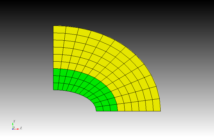

Figure 2. The affect of adjust boundary orthogonal with the snap to normal curve option is shown. The resulting mesh is orthogonal to the given boundary and projects straight through the mesh.
The following is an example of how to use this command to create the desired grid in Cubit. Note that to get the desired orthogonal grid the user must adjust the surfaces one at a time.
reset
create surface ellipse major radius 2 minor radius 1 zplane
imprint volume 1with position 0 1 0
create curve offset curve 2 distance 1 extended
create curve offset curve 4 distance 2 extended
create surface skin curve 2 4
create surface skin curve 4 5
delete surface 1
merge all
surface all scheme map
mesh surf all
adjust boundary orthogonal surface 2 snap_to_normal curve 6
adjust boundary orthogonal surface 3snap_to_normal curve 4 fixed curve 4
5.6.1.6 Centroid Area Pull
Applies to: Surface Meshes
Summary: Attempts to create elements of equal area
To create elements of equal area
On the Command Panel, click on Mesh and then Surface.
Click on the Smooth action button.
Select Centroid Area from the drop-down menu.
Enter in the appropriate values for Surface ID(s). This can also be done using the Pick Widget function.
Click Apply.
Surface <range> Smooth Scheme Centroid Area Pull [Free]
This smooth scheme attempts to create elements of equal area. Each node is pulled toward the centroids of adjacent elements by forces proportional to the respective element areas (Jones, 74).
5.6.1.7 Condition Number
Applies to: Triangular or Quadrilateral Surface Meshes, Tetrahedral or Hexahedral Volume Meshes. Does not apply to Mixed Element Meshes.
Summary: Optimizes the mesh condition number to produce well-shaped elements.
To use the condition number smoother
On the Command Panel, click on Mesh and then Surface.
Click on the Smooth action button.
Select Condition Number from the drop-down menu.
Enter in the appropriate values for Surface ID(s). This can also be done using the Pick Widget function.
Enter in the appropriate settings for Condition Number and Time (minutes).
Click Apply.
Surface <surface_id_range> Smooth Scheme Condition Number [beta <double=2.0>] [cpu <double=10>]
Discussion:
The condition number smoother is designed to be the most robust smoother in Cubit because it guarantees that if the initial mesh is non-inverted then the smoothed mesh will also be non-inverted. The price exacted for this capability is that this smoother is not as fast as some of the other smoothers.
Condition Number measures the distance of an element from the set of degenerate (non-convex or inverted) elements. Optimization of the condition number increases this distance and improves the shape quality of the elements. Condition number optimization requires that the given mesh contain no negative Jacobians. If the mesh contains negative Jacobians and this command is issued, Cubit automatically calls the Untangle smoother and attempts to remove the negative Jacobians. If successful, condition number smoothing occurs next; the resulting mesh should have no negative Jacobians. If untangling is unsuccessful, condition number smoothing is not performed.
There is no "fixed/free" option with this command; boundary nodes are always held fixed.
The command above only sets the smoothing scheme; to actually smooth the mesh one must subsequently issue the command "smooth surface <surface_id_range>" or "smooth volume <volume_id_range>".
Stopping Criteria: Smoothing will proceed until the objective function has been minimized or until one of two user input stopping criteria are satisfied. To input your own stopping criterion use the optional parameters ’beta’ and ’cpu’ in the command above. The value of beta is compared at each iteration to the maximum condition number in the mesh. If the maximum condition number is less than the value of beta, the iteration halts. In Cubit condition number ranges from 1.0 to infinity, with 1.0 being a perfectly shaped element. Thus the smaller the maximum condition number, the better the mesh shape quality. The default value of the beta parameter is 2.0. The value supplied for the "cpu" stopping criterion tells the code how many minutes to spend trying to optimize the mesh. The default value is 10 minutes. Optimization may also be halted by using "control-C" on your keyboard.
To view a detailed report of the smoothing in progress issue the command "set debug 91 on" prior to smoothing the surfaces or volumes. You will get a synopsis of whether or not untangling is needed first and whether the stopping criteria have been satisfied. In addition the following printout information is given for each iteration of the conjugate gradient numerical optimization:
iteration=n, evals=m, fcn=value1, dfmax=value2, time=value3 ave_cond=value4, max_cond=value5, min_jsc=value6
n is the iteration count, m is the number of objective function evaluations performed per iteration, value1 is the value of the objective function (this usually decreases monotonically), value2 is the norm of the gradient (does not always decrease monotonically), and value3 is the cumulative cpu time (in seconds) spent up to the current iteration. The minimum possible value of the objective function is zero but this is attained only for a perfect mesh. ave_cond, max_cond, and min_jsc are the average and maximum condition number, and the minimum scaled jacobian. ave_cond generally decreases monotonically because it is directly related to value1.
5.6.1.8 Edge Length
Applies to: Surfaces
Summary: This smoother tries to make all edge lengths equal
To use edge length smoothing
On the Command Panel, click on Mesh and then Surface.
Click on the Smooth action button.
Select Edge Length from the drop-down menu.
Enter in the appropriate values for Surface ID(s). This can also be done using the Pick Widget function.
Click Apply.
Surface <range> Smooth Scheme Edge Length
Edge Length smoothing in Cubit is provided by MESQUITE, a mesh optimization toolkit by Argonne National Laboratory and Sandia National Laboratories. (See Brewer, et al. 2003 for more details on the MESQUITE toolkit.) This smooth scheme may be useful for lengthening the shortest edge length in paved meshes.
Interior node positions are adjusted in an optimization loop where the optimal element has an ideal shape (square) and has an area equal to the average element area of the input mesh.
NOTE: This smoother should be avoided when the mesh contains high aspect-ratio elements that the user wants to keep.
Because this smoother essentially tries to make all the edge lengths equal, it is designed to work well on meshes whose elements have aspect ratios close to 1. The farther from 1 the aspect ratio is, the less applicable this smoother will be.
5.6.1.9 Equipotential
Applies to: Volume Meshes
Summary: Attempts to equalize the volume of elements attached to each node
To use edge length smoothing
On the Command Panel, click on Mesh and then Volume.
Click on the Smoothing action button.
Select Equipotential from the drop-down menu.
Enter in the appropriate values for Volume ID(s). This can also be done using the Pick Widget function.
Optionally, select Specify Tolerance to set a specific Tolerance value.
Click Apply.
Volume <range> Smooth Scheme Equipotential [Free]
This smoother is a variation of the Equipotential (Jones, 74) algorithm that has been extended to manage non-regular grids (Tipton, 90). This method tends to equalize element volumes as it adjusts nodal locations. The advantage of the equipotential method is its tendency to "pull in" badly shaped meshes. This capability is not without cost: the equipotential method may take longer to converge or may be divergent. To impose an equipotential smooth on a volume, each element must be smoothed in every iteration–a typically expensive computation. While a Laplacian method can complete smoothing operations with only local nodal calculations, the equipotential method requires complete domain information to operate.
5.6.1.10 Laplacian
Applies to: Curve, Surface, and Volume meshes
Summary: Tries to make equal edge lengths
To use laplacian smoothing
On the Command Panel, click on Mesh.
Click on Volume, Surface or Curve.
Click on the Smoothing action button.
Select Laplacian from the drop-down menu.
Enter in the appropriate values for Volume ID(s), Surface ID(s) or Curve ID(s). This can also be done using the Pick Widget function.
Optionally, select Specify Tolerance to set a specific Tolerance value.
Click Apply.
{Surface|Volume} <range> Smooth Scheme Laplacian [Free] [Global]
The length-weighted Laplacian smoothing approach calculates an average element edge length around the mesh node being smoothed to weight the magnitude of the allowed node movement (Jones, 74). Therefore this smoother is highly sensitive to element edge lengths and tends to average these lengths to form better shaped elements. However, similar to the mapping transformations, the length-weighted Laplacian formulation has difficulty with highly concave regions.
Currently, the stopping criterion for curve smoothing is 0.005, i.e., nodes are no longer moved when smoothing moves the node less than 0.005 * the minimum edge length. The maximum number of smoothing iterations is the maximum of 100 and the number of nodes in the curve mesh. Neither of these parameters can currently be set by the user.
Using the global keyword when smoothing a group of surfaces will allow smoothing of mesh on shared curves to improve the quality of elements on both surfaces sharing that curve.
5.6.1.11 Mean Ratio
Applies to: Triangular or Quadrilateral Surface Meshes, Tetrahedral or Hexahedral Volume Meshes. Does not apply to Mixed Element Meshes.
Summary: Moves interior mesh nodes to optimize the average mean ratio metric value of the mesh.
To use mean ratio smoothing
On the Command Panel, click on Mesh.
Click on Volume or Surface.
Click on the Smoothing action button.
Select Mean Ratio from the drop-down menu.
Enter in the appropriate values for Volume ID(s) or Surface ID(s). This can also be done using the Pick Widget function.
Enter the appropriate value for Time (minutes).
Click Apply.
Surface <surface_id_range> Smooth Scheme Mean Ratio [cpu <double=10>]
Volume <volume_id_range> Smooth Scheme Mean Ratio [cpu <double=10>]
Cubit includes a mean ratio smoother provided by MESQUITE, a mesh optimization toolkit by Argonne National Laboratory and Sandia National Laboratories. (See Brewer, et al. 2003 for more details on the MESQUITE toolkit.) This smoother is similar in purpose to the Condition Number smoother. However, the Mean Ratio smoother uses a second order optimization method, and therefore it will often reach a near-optimal mesh more quickly than the Condition Number smoother. The Mean Ratio smoother requires the initial mesh to be untangled, but the smoother is guaranteed to not tangle the mesh. If the user attempts to call the Mean Ratio smoother on a tangled mesh, an untangler will first attempt to untangle the mesh before calling the Mean Ratio smoother.
The Mean Ratio smoother’s optimization process terminates when one of the following three criteria is met:
The mesh is "close" to an optimal mesh configuration.
The maximum allotted time has been exceeded.
The user interrupts the smoothing process.
The user has control over the second and the third criteria only. For criterion 2, the default is for the smoother to terminate after ten minutes even if a near-optimal mesh has not been reached. The user can change this time bound by specifying the optional "cpu" argument in the command listed above. This argument takes a single, positive number that represents the time (in minutes) that will be used as a time bound. If the user wishes to terminate the process early, criteria three allows the user to "interrupt" (for example, on some platforms, by pressing CTRL-C) the process. If the process is terminated early, the mesh will not revert to the original node positions; Cubit will instead keep the partially optimized mesh.
5.6.1.12 Smart Laplacian
Applies to: Surface and Volume meshes
Summary: Tries to make equal edge lengths while ensuring no degradation in element shape
To use smart laplacian smoothing
On the Command Panel, click on Mesh.
Click on Volume or Surface.
Click on the Smoothing action button.
Select Smart Laplacian from the drop-down menu.
Enter in the appropriate values for Volume ID(s) or Surface ID(s). This can also be done using the Pick Widget function.
Click Apply.
{Surface|Volume} <range> Smooth Scheme Smart Laplacian
The Smart Laplacian smoothing approach is a variation on the standard Laplacian algorithm. The algorithm iteratively loops over the mesh and updates nodes based on the location of their neighbors. First, a patch of elements is formed around a given node. The quality of this patch is assessed to determine the quality of the worst shaped element. Then a new candidate node position is calculated as the average of the neighboring nodes. The quality of the patch is assessed again using the candidate node position. If there has been no degradation in the quality of the elements in the patch, the candidate node position is accepted; otherwise, the candidate node position is rejected and the node is returned to its previous position.
The Smart Laplacian smoother is intended to provide a reliable smoother that is nearly as fast as the Length-Weighted Laplacian smoother. Due to the dual goals of this smoother, making equal edge length and improving element shape, it will not always be able to make progress. However, it is often useful as a quick alternative to the more time-consuming optimization methods like Mean Ratio or Condition Number. When this smoother fails to make significant progress, the optimization methods can be tried.
The Smart Laplacian Smoother uses the Mean Ratio quality measure to assess element shape. This smoother is ensuring no degradation in the minimum Mean Ratio. The Mean Ratio smoother is optimizing the same metric, but it is attempting to improve the average Mean Ratio quality.
5.6.1.13 Untangle
Applies to: Triangular or Quadrilateral Surface Meshes Tetrahedral or Hexahedral Volume Meshes. Does not apply to Mixed Element Meshes.
Summary: Removes as many negative Jacobians from the mesh as possible by minimizing a certain objective function.
To use untangle smoothing
On the Command Panel, click on Mesh.
Click on Volume or Surface.
Click on the Smoothing action button.
Select Untangle from the drop-down menu.
Enter in the appropriate values for Volume ID(s) or Surface ID(s). This can also be done using the Pick Widget function.
Enter the appropriate values for Scaled Jacobian and Time (minutes).
Click Apply.
Surface <surface_id_range> Smooth Scheme Untangle [beta <double=0.02>] [cpu <double=10>]
Volume <volume_id_range> Smooth Scheme Untangle [beta <double=0.02>] [cpu <double=10>]
Discussion:
The Untangle ’smoother’ is designed to eliminate negative Jacobians from a given mesh by moving nodes to appropriate locations. If a mesh node is not involved in causing a negative Jacobian it will not be moved. If a mesh has no negative Jacobians, the Untangler will not move any of the nodes. This smoother is not magic: if an untangled mesh does not exist for the given mesh topology, the untangler will not untangle the mesh. Instead, it will do the best it can and exit gracefully. An untangled mesh produced by this smoother will often have poor shape quality; in that case it is recommended that untangling be followed by condition number smoothing. The untangle smoother is automatically called by the condition number smoother.
There is no "fixed/free" option with this command; boundary nodes are always held fixed. As a result, users should be aware that the volume untangler cannot succeed if the volume contains a surface mesh which contains a negative Jacobian. In that case, one must first remove the surface mesh negative Jacobians by invoking the surface Untangler and then invoke the volume Untangler.
The command above only sets the smoothing scheme; to actually smooth the mesh one must subsequently issue the command smooth surface <surface_id_range> or smooth volume <volume_id_range>.
Stopping Criteria: Untangling will proceed until the objective function has been minimized or the optional user input cpu has been satisfied. The latter stopping criterion tells the code how many minutes to spend trying to untangle the mesh. The default value is 10 minutes. Optimization may also be halted by using "control-C" on your keyboard.
Beta Parameter: An optional user input parameter beta plays a role in determining the optimal mesh. Optimization proceeds until the minimum scaled Jacobian of the mesh is (roughly) greater than beta. To remove negative Jacobians one would need beta=0 (however, as a safety margin, we choose beta=0.02 as the default). To further improve the scaled Jacobian of the mesh, input a larger value of "beta". If a mesh with all scaled Jacobians greater than "beta" does not exist, optimization will continue until the cpu time stopping criterion has been met. Therefore, it is best not to use "beta" values too large (say, greater than 0.2) without also decreasing the cpu time limit.
Iteration=n, Evals=m, Fcn=value1, dfmax=value2, time=value3 min_jsc=value4
5.6.1.14 Winslow
Applies to: Surface meshes
Summary: Elliptic smoothing technique for structured and unstructured surface meshes
To use winslow smoothing
On the Command Panel, click on Mesh and then Surface.
Click on the Smooth action button.
Select Winslow from the drop-down menu.
Enter the appropriate values for Surface ID(s). This can also be done using the Pick Widget function.
Click Apply.
Surface <range> Smooth Scheme Winslow [Free]
Winslow elliptic smoothing (Knupp, 98) is based on solving Laplaces equation with the independent and dependent variables interchanged. The method is widely used in conjunction with the mapping and submapping methods to give smooth meshes with positive Jacobians, even on non-convex two-dimensional regions. The method has been extended in Cubit to work on unstructured meshes.
5.6.2 Align Mesh
Align Mesh Surface <id> [CloseTo] Surface <id> [Tolerance <tol>]
Align Mesh Curve <id> [CloseTo] Curve <id> [Tolerance <tol>]
Align Mesh Node <id> [CloseTo] Node <id> [Tolerance <tol>]
And example of this is given as follows:
brick x 10
volume 1 copy move 11
surface all except 10 6 vis off
transparent
graphics perspective off
at 5.552503 3.832384 0.134127
from 34.651051 3.640138 -0.193121
up 0.006514 0.999945 -0.008172
mesh surface all
surface 6 smooth scheme randomize free
smooth surface 6
node 432 move 0 0 -0.2
align mesh node 944 node 432
node 432 move 0 0 0.4
align mesh curve 23 closeto curve 12
align mesh surf 10 closeto surf 6
5.6.3 Block Repositioning
Block <id_range> Move <delta_x><delta_y><delta_z>
5.6.4 Collapsing Mesh
CUBIT currently offers several options for modifying an existing finite element mesh. Triangle and tetrahedral meshes sometimes contain low quality elements that can be removed by the following operations.
5.6.4.1 Collapsing Mesh Using Quality Metrics
Collapse Edge <ids> [SCALED JACOBIAN|Aspect Ratio|Shape|Shape and Size]
Collapse Tri <ids> [SCALED JACOBIAN|Aspect Ratio|Shape|Shape and Size]
Collapse Tet <ids> [Altitude|Aspect Ratio|Aspect Ratio Gam|Distortion|Inradius|Jacobian|Normalized Inradius|Node Distance|SCALED JACOBIAN|Shape|Shape and Size|Timestep]
5.6.4.2 Collapsing Mesh Manually
Meshedit Collapse edge <id> [keep node <id>] [compress_ids]
Merge Node <id> <id>
5.6.4.3 Removing Overconstrianed Tets
Remove Overconstrained Tet <ids>
5.6.5 Creating and Merging Mesh Elements
The following forms of the create and merge commands operate on meshed entities only. They allow low-level editing of meshes to make minor corrections to a mostly correct mesh. They are not designed for major modifications to existing meshes. Because Cubit’ display routines were not designed with these type of operations in mind, these commands may cause the current display of the affected entities to take an unexpected form. An appropriate drawing command can be used to return the display to the desired view.
The delete commands for deleting individual elements are still under development, but they may be used after setting a developer flag.
5.6.5.1 Creating Mesh Elements
The create command uses existing mesh nodes to create new mesh entities.
5.6.5.1.1 Creating Hex and Tet Elements
To create hex and tet elements using existing mesh nodes
On the Command Panel, click on Mesh.
Click on Hex or Tet.
Click on the Create action button.
Enter the appropriate value for each Node ID.
Enter the appropriate value for Volume ID. This can also be done using the Pick Widget function.
Click Apply.
Create {Hex|Tet} Node <range> [Owner Volume <id>]
create hex node 1,2,3,4,5,6,7,8 owner volume 1
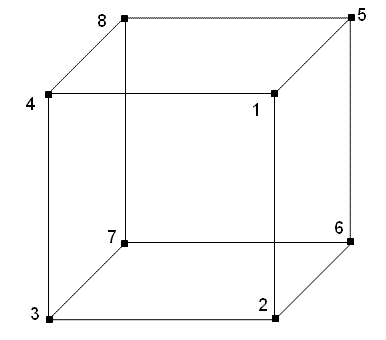
create tet node 1,2,3,4 owner volume 1
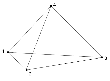
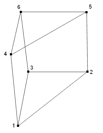
5.6.5.1.2 Creating Wedge Elements
Create Wedge Node <range> [Owner Volume <id>]
create wedge node 1,2,3,4,5,6 owner volume 1
5.6.5.1.3 Creating Face and Tri Elements
To create quad and tri elements using existing mesh nodes
On the Command Panel, click on Mesh.
Click on Quad or Tri.
Click on the Create action button.
Select Single Element from the drop-down menu.
Enter the appropriate value for each Node ID.
Enter the appropriate value for Volume ID. This can also be done using the Pick Widget function.
Click Apply.
Create {Face|Tri} Node <range> [Owner {Volume|Surface} <id>]
5.6.5.1.4 Creating Edge Elements
To create edge elements using existing mesh nodes
On the Command Panel, click on Mesh.
Click on Edge.
Click on the Create action button.
Select Single Element from the drop-down menu.
Enter the appropriate value for each Node ID.
Enter the appropriate value for Volume ID. This can also be done using the Pick Widget function.
Click Apply.
Create Edge Node <range> [Owner {Volume|Surface|Curve} <id>]
5.6.5.1.5 Creating Nodes
To create a node by specifying the location
On the Command Panel, click on Mesh and then Node.
Click on the Create action button.
Specify the X, Y and Z Coordinates.
Choose a Node Owner by selecting Volume, Surface, Curve or Vertex from the Node Owner drop-down menu.
Enter the appropriate value for the selected Node Owner. This can also be done using the Pick Widget function.
Click Apply.
Create Node Location <x> <y> <z> Owner {Volume|Surface|Curve|Vertex} <id>
5.6.5.2 Merging Nodes
Merge Node <id1> <id2>
Caution should be taken when using the merge node command because other commands involving the related meshed entities may not work properly following the merge.
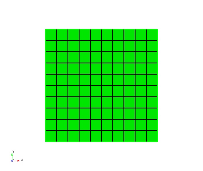
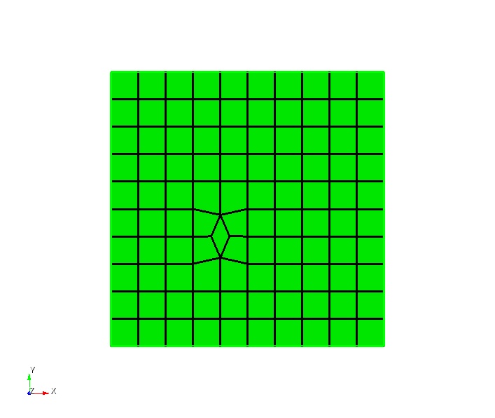
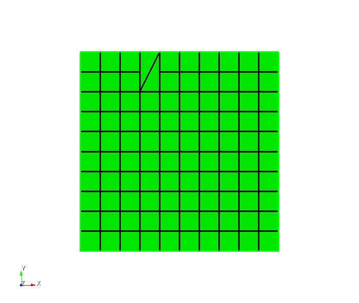
5.6.6 Edge Swapping
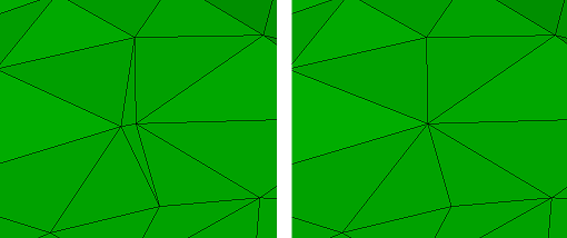
The edge swap command allows a user to target a specific edge between two triangles (similar functionality for quads and tets has not been included) and change the connectivity of the triangles.Multiple edges can be swapped simultaneously. The input order of the edges is the order in which the swaps will be performed.
Typically, the edge swap command is used to specifically repair local mesh connectivity.
Swap Edge <id_list>
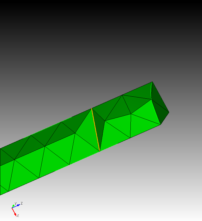
Image 1 - Before edge swapping
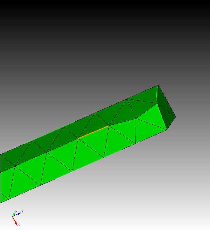
Image 2 - After edge swapping
5.6.7 Matching Tetrahedral Meshes
The intended use of this function is for importing two exodus or genesis files that have non-conforming mesh where they touch and modifying the meshes locally to make them conforming.The result is a single mesh that is stitched together at the locally modified region. This functionality is currently only available for tetrahedral meshes.
Tetrahedral mesh matching will work on free mesh only.The interface where the two meshes will be matched need not be planar.A single target sideset and one or more source sidesets should be provided. The source sideset should be completely enclosed in the target sideset so that the boundaries of the two sidesets do not intersect. The two meshes need not touch exactly at the sidesets but the closer the meshes are to touching the better the results will be.Small gaps or overlaps will generally be allowed.Both of the meshes involved in the matching should be contained in defined blocks prior to issuing the command.
Meshmatch tet sideset <id_list> onto sideset <id>
The one or more sidesets specified before the onto keyword are the source sideset(s). The sideset after the onto keyword is the target sideset.
5.6.8 Mesh Cleanup
Cleanup {Volume|Block <id_range>} [angle <value=150>]
5.6.8.1 Cleaning Up a Tetrahedral Mesh
An alternative to the remesh command for tetrahedral meshes is the cleanup command. For this command the existing mesh is validated and "optimized" by the tetmesher, instead of being deleted and replaced with a different mesh.
Cleanup {Volume|Block} <id_range>
cleanup tet <id_range> [free]
For example, the command
cleanup tet all free
Also, the command
cleanup tet 200 to 300
Note: Cubit will issue an error if the tetrahedra are owned by more than one volume or mesh container.
5.6.8.2 Cleaning Up a Hexahedral Mesh
Cleanup Volume <id_range> [angle <value=150>]
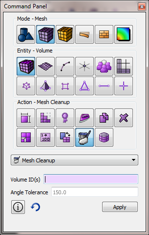
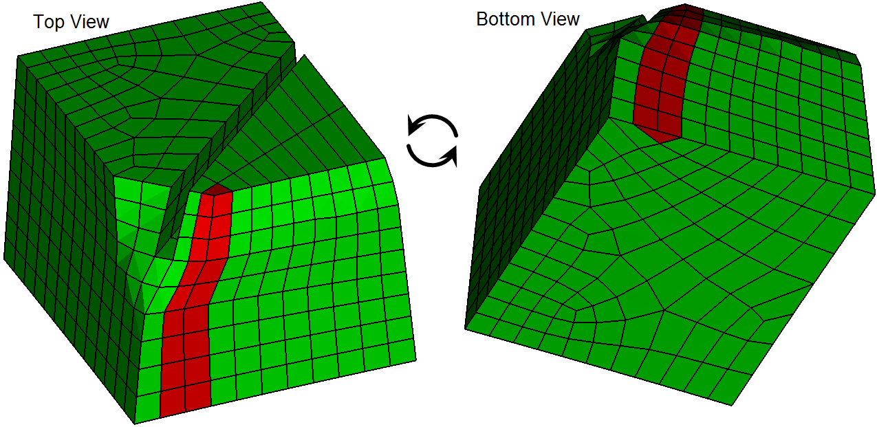
Figure 387: The mesh from Figure 386 after hex mesh cleanup.
5.6.9 Mesh Coarsening
5.6.9.1 Hexahedral Coarsening
Cubit provides a limited number of options for coarsening hexahedral meshes. The options currently available for hex coarsening rely on the hex sheet extraction process described in Mesh Refinement page. Removing a sheet from a hexahedral mesh essentially means that a complete layer of hexes will be removed and the adjacent layers expanded to take its place.
5.6.9.1.1 Extracting a Single Hex Sheet
Extract sheet { Edge <id> | Node <id_1> <id_2> }
Note: Also see the Mesh Refinement section for a description of hex sheet drawing.
5.6.9.1.2 Extracting multiple sheets along a curve
Coarsen Mesh Curve <id> Factor <value> [NO_SMOOTH|smooth]
Coarsen Mesh Curve <id> Remove {<num_edges>|edge <id_ranges>} [NO_SMOOTH|smooth]
The first option uses the factor argument. The factor argument controls how much larger the edges will be on the curve. For example, Figure 389 shows the coarsen mesh curve command used with a factor of 2. In this case, the command attempts to make the mesh edges approximately twice the length relative to their original length along the curve.
The second option uses the remove argument. With this option, a specified number of layers may be removed from the mesh. This may be accomplished by indicating an exact number, or by providing a list of edge IDs that correspond to the layers that will be removed.
The NO_SMOOTH|smooth option allows the user to improve the element quality after the sheet extraction process by smoothing the remaining nodes. The default for both of these commands is to not smooth. Smoothing may also be accomplished after sheet extraction by using the smooth volume command.
5.6.9.1.3 Uniform hex coarsening
By applying the coarsen mesh curve command multiple times to curves that are orthogonal in the model, the effect of uniform coarsening of the mesh may be achieved.
5.6.10 Mesh Column Operations
Column operations allow users direct control over the mesh connectivity while maintaining full-geometric associativity. Often, hex meshing schemes such as sweeping and mapping result in mesh topology forced into unnatural shapes, such as a square shaped source surface mesh getting swept into a circular target surface. Often forcing meshes into shapes like this results in poor element quality because of non-optimal element angles. The Column commands allow users to directly modify mesh topology to make minor tweaks to a mesh improving element quality. Column operations are almost always followed by smoothing to enable element quality improvement. Cubit provides tools to perform insertion, deletion, swapping, grouping, and drawing of hex columns.
5.6.10.1 Column Insertion
column open node <center node id> <orientation node ids>
5.6.10.2 Column Deletion
Columns can be removed with neighboring columns being joined together using collapse commands. Collapse commands are of two types: interior and boundary.
column collapse node <opposite node ids>
5.6.10.3 Column Swapping
column swap node <old edge node ids> <new edge node ids>
5.6.10.4 Column Groups
column { face <id> | edge <id1> <id2> | hex <id1> <id2> } group
5.6.10.5 Drawing Columns
draw column { face <id> | edge <id1> <id2> | hex <id1> <id2>}
5.6.11 Mesh Refinement
Cubit provides several methods for conformally refining an existing mesh. Conformal mesh refinement does not leave hanging nodes in the mesh after refinement operations, rather conformal mesh refinement provides transition elements to the existing mesh. Both local and global mesh refinement operations are provided.
5.6.11.1 Global Mesh Refinement
Refine Volume <range> numsplit <int>
Refine Surface <range> numsplit <int>
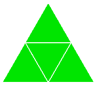
original mesh
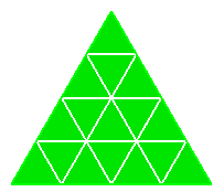
NumSplit = 1
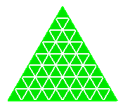
NumSplit = 2
original mesh
NumSplit = 1
NumSplit = 2
original mesh
NumSplit = 1
NumSplit = 2
original mesh
NumSplit = 1
NumSplit = 2
Figure 397: Example of uniform refinement for each of the mesh entities
5.6.11.2 Refining at a Geometric or Mesh Feature
Refine {Node|Edge|Tri|Face|Tet|Hex} <range>
[NumSplit<int = 1>|Size <double> [Bias <double>]]
[Depth <int>|Radius <double>] [Sizing_Function]
[Smooth]
Refine {Vertex|Curve|Surface} <range>
NumSplit<int = 1>|Size <double> [Bias <double>]]
[Depth <int>|Radius <double>] [Sizing_Function]
[Smooth]
The following is a description of refinement options.
Numsplit
Defines the number of times the refinement operation will be applied to the elements in the refinement region. For uniform or global refinement, where all elements in the model are to be refined, A NumSplit value of 1 will split each triangle and quadrilateral into four elements, and each tetrahedron and hexahedraon into eight elements. A numsplit of 2 would result in 9 and 27 elements respectively. For uniform refinement, the total number of elements obeys the following:
NE = NI * (numsplit + 1)^dim
where NE is the final number of elements, NI is the initial number of elements and dim is 2 or 3 for 2D and 3D elements respectively.
In cases where only a portion of the elements are selected for refinement, the elements at the boundary between the refined and non-refined elements will be split to accommodate a transition in element size. The transition pattern will vary depending on the local features and surrounding elements. For non-uniform refinement of hexahedron, for a numsplit of 1, each element in the uniform refinement zone will be subdivided into 27 elements rather than 8. This affords greater flexibility in transitioning between the refined and unrefined elements.
The Size and Bias options are useful when a specific element size is desired at a known location. This might be used for locally refining around a vertex or curve. The Bias argument can be used with the Size option to define the rate at which the element sizes will change to meet the existing element sizes on the model. Figure 398 shows an example of using the Size and Bias options around a vertex. Valid input values for Bias are greater than 1.0 and represent the maximum change in element size from one element to the next. Since refinement is a discrete operation, the Size and Bias options can only approximate the desired input values. This may cause apparent discontinuities in the element sizes. Using the default smooth option can lessen this effect. It should also be noted that the Size option is exclusive of the NumSplit option. Either NumSplit or Size can be specified, but not both.
original mesh
Bias=2.0
Bias=1.5
Figure 398: Example of using the Size and Bias options at a Vertex.
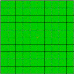
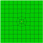
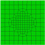
The Depth option permits the user to specify how many elements away from the specified entity will also be refined. Default Depth is 1. Figure 399 shows an example of using the depth option when refining at a node.
original mesh
Depth=1
Depth=2
Figure 399: Example of using the Depth option at a node to control how far from the node to propagate the refinement.
Instead of specifying the number of elements to describe how far to propagate the refinement, a real Radius may be entered. The effects of the Radius are similar to that shown in Figure 3, except that the elements whose centroid fall within the specified Radius will be refined. Transition elements are inserted outside of this region to transition to the existing elements.
Refinement may also be controlled by a sizing function. Cubit uses sizing functions to control the local density of a mesh. Various options for setting up a sizing function are provided, including importing scalar field data from an exodus file. In order to use this option, a sizing function must first be specified on the surface or volume on which the refinement will be applied. See Adaptive Meshing for a description of how to define a sizing function.
Smooth
The default mode for refinement operations is to NOT perform smoothing after splitting the elements. In many cases, it may be necessary to perform smoothing on the model to improve quality. The smooth option provides this capability.
Controlling Regularity of Triangle Refinement
The default behavior of triangle refinement is to attempt to maximize element quality using the basic one->four template. This can sometimes result in an irregular pattern, where one or more edges are swapped. To enforce regularity of the triangle refinement pattern, regardless of quality, the folowing setting may be used.
Set Triangle Refine Regular {on|OFF}
5.6.11.3 Hexahedral Refinement Using Sheet Insertion
Several tools for refining a hexahedral mesh using sheet insertion and deletion are available in Cubit.
5.6.11.3.1 Refining at a Geometric Feature
The following commands offer additional controls on refinement with respect to one or more geometric features of the model.
Refine Mesh Volume <id> Feature {Surface | Curve | Vertex | Node} <id_range> Interval <integer>
Figure 400 shows an example of this command where the feature at which refinement is to be performed is a curve. In this case the interval chosen was, 2. This indicated that the elements 2 intervals away from the curve would be refined.
5.6.11.3.2 Refining along a path
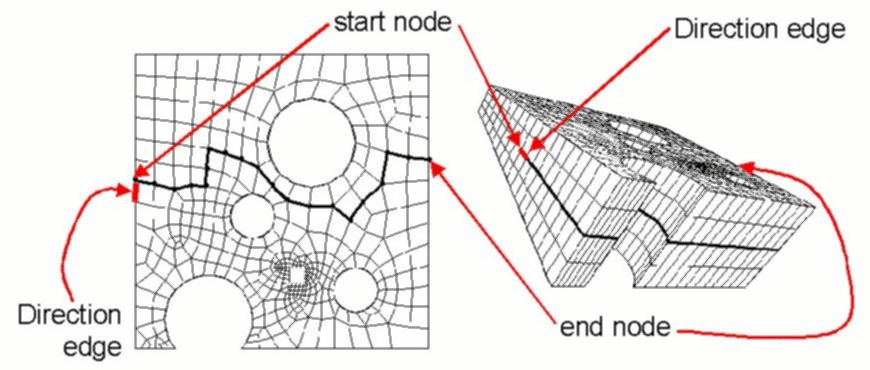
Refine Mesh Start Node <id> Direction Edge <id> End Node <id> [Smooth]
5.6.11.3.3 Refining a Hex Sheet
Refine Mesh Sheet [Intersect] { Node <id_1> <id_2> | Edge <id_range> } { Factor <double> | Greater_than <size> } [Smooth] [in volume <id_range> [depth <num_layers]]
Figure 403: Refine mesh sheet edge 1584 1564 1533 1502 1471 greater_than 6
The factor and greater_than keywords are used to specify the refinement criteria for the selected hex sheet(s). If the factor keyword is used, the length of the smallest edge in the hex sheet is determined and any edge in the hex sheet with a length greater than the smallest length multiplied by the factor is refined. If the greater_than keyword is used, any edge in the hex sheet with a length greater than the specified size is refined.
The intersect keyword is optional. It is used to more easily define multiple hex sheets to be refined. If the intersect keyword is entered, the node and edge keywords are used to define a chord rather than a sheet (a chord is the two-dimensional equivalent of the three-dimensional sheet). The chord will be limited to the surface(s) associated with the nodes or edge entered, and all sheets intersecting the chord will be selected for refinement (see Figure 404). When the node keyword is used with the intersect option, the nodes must define an edge on the surface of the mesh.
Figure 404: Refine mesh sheet intersect edge 1499 greater_than 6
The smooth keyword is also optional. When the smooth keyword is entered, the elements that have been refined are smoothed in an attempt to improve element quality. Figure 405 shows the same command as Figure 404 with the addition of the smooth keyword. Smoothing may or may not be beneficial, depending on the situation.
Figure 405: Refine mesh sheet intersect edge 1499 greater_than 6 smooth
5.6.11.3.4 Directional Refinement
Mesh sheet refinement can also be used to refine a mesh in a particular direction.This can help control anisotropy.The following command can be used as a short cut for specifying what sheets should be used in refinement.
Refine Volumes <id_range> using {Plane <options> | Surface <id_range> | Curve <id_range> } [ Depth <num_layers> ] [ Smooth ]
refine vol 2 using plane xplane depth 1

Figure 407: Directional result of refinement resulting from using the plane option on the refinement command.
refine mesh sheet edge ( at 4.5 5 5 ordinal 1 ) factor 0
refine vol 2 using plane xplane depth 1
Figure 408: A 2nd iteration of direction refinement is applied.
5.6.11.3.5 Hex Sheet Drawing
Since refinement of hex meshes generally occurs by inserting hex sheets, tools have been provided to draw a specified sheet or group of sheets.
Draw Sheet {Edge <id> |Node <id_1> <id_2>}[Mesh [List]] [Color <color_name>] [Gradient]
Draw Sheet Hex <id> [Green][Yellow][Red][Mesh [List]] [Gradient]
The ’mesh’ keyword will draw the hexes in the hex sheet. If the ’list’ keyword is also given, the ids of the hexes in the sheet will be listed.
5.6.11.4 Local Refinement of Tets, Triangles, and Edges
Local refinement of tets, triangles, and edges is available by refining individual entities or by refining to guarantee a user-specified number of tests through the thickness:
5.6.11.4.1 Single Entity Refinement
Refine Local Tri <tri_id_list>
Refine Local Edge <edge_id>
Refine Tet_edge Node <node1_id> <node2_id>
5.6.11.4.2 ’N’ Tets Through the Thickness Refinement
Refine min_through_thickness <val> source {surface|node|tri|nodeset|sideset|block} <id_range> target {surface|node|tri|nodeset|sideset|block} <id_range> [anisotropic] [single_iteration] [dont_fill_in_gaps]
anisotropic: When this option is specified in the command the algorithm will only attempt to refine the edges that go roughly normal to the source and target entities. This will give an anisotropic result. The meshes on the source and target will generally not be affected when this option is used. When this option is not specified the refinement algorithm will be isotropic in nature and will propagate much more. However, it will tend to have better transitioning from the refined region to the non-refined regions.
dont_fill_in_gaps: When this option is specified in the command the algorithm will NOT try to grow the regions that will be refined. When the regions are grown it helps to avoid leaving small pockets of mesh that are not refined (splotchiness). This has effect only on isotropic refinement (when the "anisotropic" option is NOT used).
single_iteration: When this option is specified in the command the algorithm will only run for one iteration even if the min_through_thickness criteria is not met.
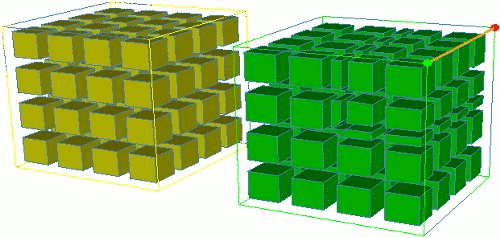
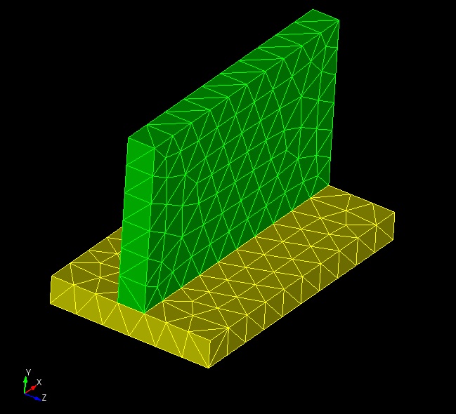
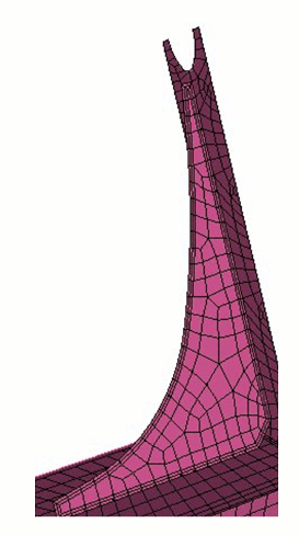
Below is an example using the following commands:
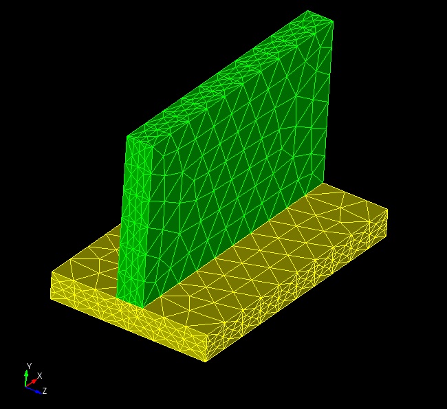
refine min_through_thickness 4 source surf 1 target surf 2 anisotropic
refine min_through_thickness 4 source surf 7 target surf 13 3 14 anisotropic
Surfaces 1 and 2 are the two surfaces on opposite sides of the thin region in the green volume and surfaces 7 13 3 14 are the surfaces on opposite sides of the thin region in the yellow volume.
5.6.11.5 Parallel Refinement
Refine Parallel [Fileroot <’root filename’>] [Overwrite] [No_geom] [No_execute] [Processors <int>] [Numsplit <int>] [Version <’Sierra version’>]
When the mesh is refined in STK_Adapt, the new nodes created during refinement will be projected to the geometry definitions from the OpenNURBS file. If the no_geom argument is specified, only the Exodus file is written, and new nodes will be placed by evaluating the shape functions of the elements being evaluated.
The exported Exodus and OpenNURBS files are prepared specifically for input into the Sierra STK_Adapt program. By default, Cubit spawns STK_Adapt in the background after exporting the files. If the no_execute argument is specified, the Cubit command exports the files, but does not spawn STK_Adapt. The user can then move those files to a large parallel machine to perform the STK_Adapt refinement.
If no_execute is not specified, then Cubit will spawn Sierra STK_Adapt in the background to perform the refinement. The processors argument specifies the number of processors to use for the STK_Adapt run. The numsplit argument specifies how many times the global refinement should be performed. If numsplit = 1, then each element edge is split into 2 sub-edges. If numsplit = 2, then each element is split into 4 sub-edges, etc. The optional version argument allows the user to specify which version of STK_Adapt should be run. Possible values for version include "head", "4.22.0", etc.
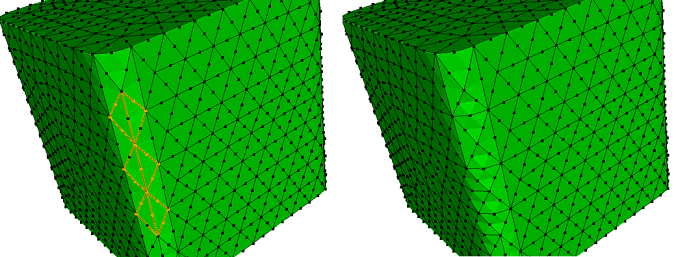
Refine parallel command creates groups to visualize the association between mesh entities (edge, tri, and quads ) and geometric entities (curves & surfaces). There are three types of groups that exist for each mesh entity type edge, tri, and quad. First group contains unique 1-1 map between mesh entity and geometric entity. Note that issuing "Debug 212" command before calling the refine parallel command, will create separate group for each geometric entity containing unique mesh entities. Next group contains mesh entities that point to multiple geometric entities. And the final group contains mesh entities not associated with any geometric entity.
After the Refine Parallel command finishes, the mesh in Cubit does not change, normally because the resulting mesh would be too big to store in Cubit on a single processor. Instead, the refined mesh is written to disk in a series of Exodus files, one per processor, using the fileroot argument as the root of the Exodus file names. For example, if fileroot is somemesh and processors is 8, STK_Adapt will write out eight Exodus files named somemesh.e.8.0, somemesh.e.8.1, ..., somemesh.e.8.7. These files can be kept distributed for an analysis run, or united using the Sierra EPU command. In this example, Cubit would have written out a file called somemesh.in.e, which contains all of the sideset, nodeset, and block definitions defined in the Cubit session. All of these sidesets, nodesets and blocks are transferred to the refined exodus files (somemesh.e.8.0, etc.) for use in the subsequent analysis. The somemesh.e.* files will also contain several other blocks which correspond to geometric entities defined in somemesh.3dm to enable the mesh to be refined to the CAD geometry, and should be ignored by downstream applications.
Sierra STK_Adapt must be in the PATH on the computer Cubit is running on. If Sierra STK_Adapt cannot be found, Cubit returns an error and no refinement is performed. Information on how to download and build Sierra STK_Adapt can be found at https://github.com/trilinos/Trilinos/tree/master/packages/stk/ .
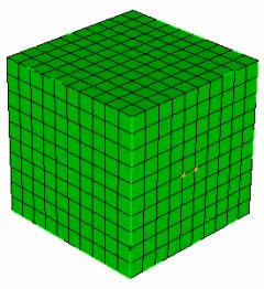
5.6.12 Mesh Scaling for Flexible Hex Refinement
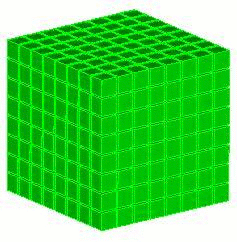
Mesh Scaling is a tool to globally refine or coarsen a hexahedral mesh. (It only works on all-hex meshes.) Mesh Scaling is more flexible than template-based global refinement methods, because it does not require that every element is refined, or refined in the same way. Instead, Mesh Scaling decomposes the entire mesh into larger "blocks" of hexes, and then refines the blocks. In this way, Mesh Scaling supports increasing the element count by small multiplicative factors, e.g. 1.5, that are impossible with template based refinement. However, like template refinement, it can ensure that every location of the mesh is refined. These features can be useful for solution verification.
Mesh Scaling allows a series of meshes to be built for solution convergence studies, or other purposes. Each mesh has similar structure but progressively smaller elements. For example, if the input mesh has 10,000 hexahedra, scaling with a multiplier of 2.0 will result in a mesh of about 20,000 hexahedra, with approximately the same element orientation and size gradations as the original. Additional meshes can be built by scaling the original mesh with multipliers of 4, 6, 8, etc. Convergence studies can be performed with much less computational cost than if traditional global refinement is used, because the element increase at each step of the series can be smaller.
A traditional template-based refinement replaces each hexahedron with a 2x2x2 structured grid of hexahedra, increasing the element count by a factor of 8X. In contrast, Mesh Scaling refines "blocks" of elements (not to be confused with Exodus element blocks). The block decomposition subdivides the entire mesh into structured (mapped) and swept blocks. A block may contain many elements, but is not allowed to cross geometric boundaries, boundary conditions, and loading constraints. For example, a block cannot have a curve or nodeset in its interior, nor hexes from multiple Exodus blocks. Blocks may be structured or logical sweeps. A structured block is restricted to be a grid of MxNxO hexes, so, its extent is limited by any surface nodes that do not have exactly four edges, etc. Mesh Scaling remeshes the entire model conforming to the block decomposition, using the original mesh as a sizing function, multiplied by the scale factor.
scale mesh [volume <ids>]
[multiplier <value, default=2.0>]
[minimum <value, default=1>]
[{SWEPT_BLOCKS | legacy | maintain_structure}]
[feature_angle <value>]
[force_structured in {[volume <ids>] [surface <ids>]}]
[thin_gap_intervals <value, default=2>] [fix_all_gaps]
[max_aspect_ratio <value> in volume <ids>]
[max_feature_length <value, default=30>]
[smooth_volume {ON|off}]
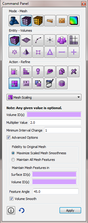
The GUI command panel for this command can be found under Mesh/Volume/Refine/Mesh Scaling.
5.6.12.1 Command Options
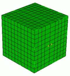
scale mesh [volume <ids>]
[multiplier <value, default=2.0>]
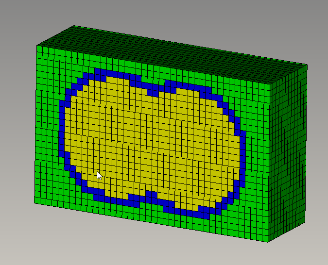
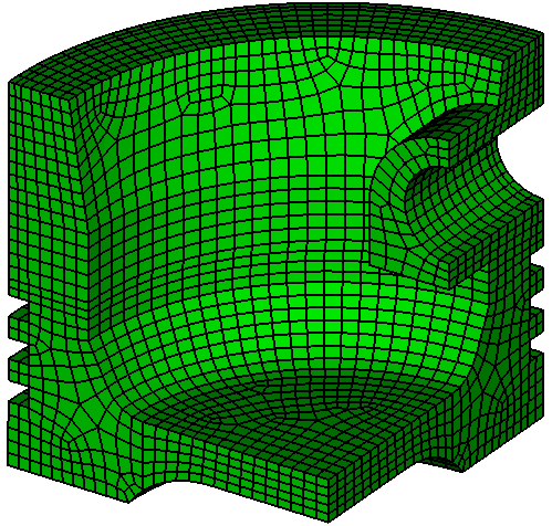
Figure 413: The mesh from Figure 412 scaled with the command "Scale Mesh Multi 2". The resulting mesh contains 6804 hex elements.
[minimum <value, default=1>]
5.6.12.1.1 Refinement and Coarsening Levels
The multiplier determines the target number of output hexes. There is no guarantee it will be achieved exactly. Mesh Scaling will output at least multiplier*n hexes, where n is the number of input hexes. For minimum 0 and small multipliers there is no guarantee that every block will be refined in all 3 directions. This is because the target number of elements may be reached first. This may lead to unevenly distributed refinement with jumps in adjacent element sizes.
An uneven distribution may also result if adjacent blocks have significantly different MxNxO intervals; this is common with the legacy option. For example, for a 1x10x12 block adjacent to a 6x10x12 block, Mesh Scaling could output 2x11x13 and 7x11x13 blocks. The M value of the first block has doubled, 2/1, while the M value of the second block has only increased by 7/6. Thus, the user may observe a jump in the lengths of adjacent edges.
To coarsen a mesh, specify a multiplier less than one. Mesh scaling will output at most multiplier*n hexes. For example, a multiplier of 0.9 will attempt to decrease the element count by 10%. Each block side will have its intervals decreased by the minimum value. A block must have at least one interval, so how far the mesh can be coarsened is limited by the distance between mesh irregularities, geometry, boundary condition and loading constraints.
5.6.12.1.2 Solution Verification
(2X, 1) (4X, 2) (8X, 3) (16X, 4), (prior *2, prior +1), etc.
(2X, 1) (3X, 1) (4X, 2) (5X, 2) (6X, 2) (7X, 2) (8X, 3) etc..
[{SWEPT_BLOCKS | legacy | maintain_structure}]
The block decomposition options are swept_blocks (default), maintain_structure and legacy. For legacy, only structured blocks are used. For swept_blocks and maintain_structure, the decomposition constructs large swept blocks wherever logical sweeps can be identified, and structured blocks otherwise. The main difference is that swept_blocks remeshes the source surfaces of swept blocks from scratch. In contrast, maintain_structure partition each swept block into structured sub-blocks, and remeshes by selectively refining those sub-blocks. Thus swept_blocks may change the number and relative location of irregular nodes, whereas maintain_structure keeps them the same.
Typically, swept_blocks and maintain_structure provide smoother, more evenly distributed refinements compared to legacy. This is because with swept blocks there are typically significantly fewer blocks in the decomposition. Having fewer blocks increases the likelihood that each block will receive at least some refinement before the multiplier is reached.
However, legacy and maintain_structure provide element orientations and structure closer to the original mesh than swept_blocks. This is because structured blocks maintain the irregular nodes.
Often maintain_structure provides both element orientations closer to the original mesh and a smoother, more evenly distributed refinement. Its structured blocks preserve orientations and structure. Its swept blocks provide the freedom to distribute changes, and smooth the mesh, across its structured sub-blocks.
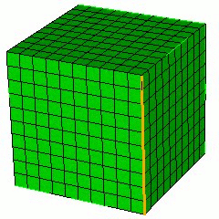
[force_structured in {[volume <ids>] [surface <ids>]}]
Figure 414: Input mesh for Mesh Scaling. Surface 108 contains a non-mapped, but still structured mesh. Surface 34 contains a paved mesh.
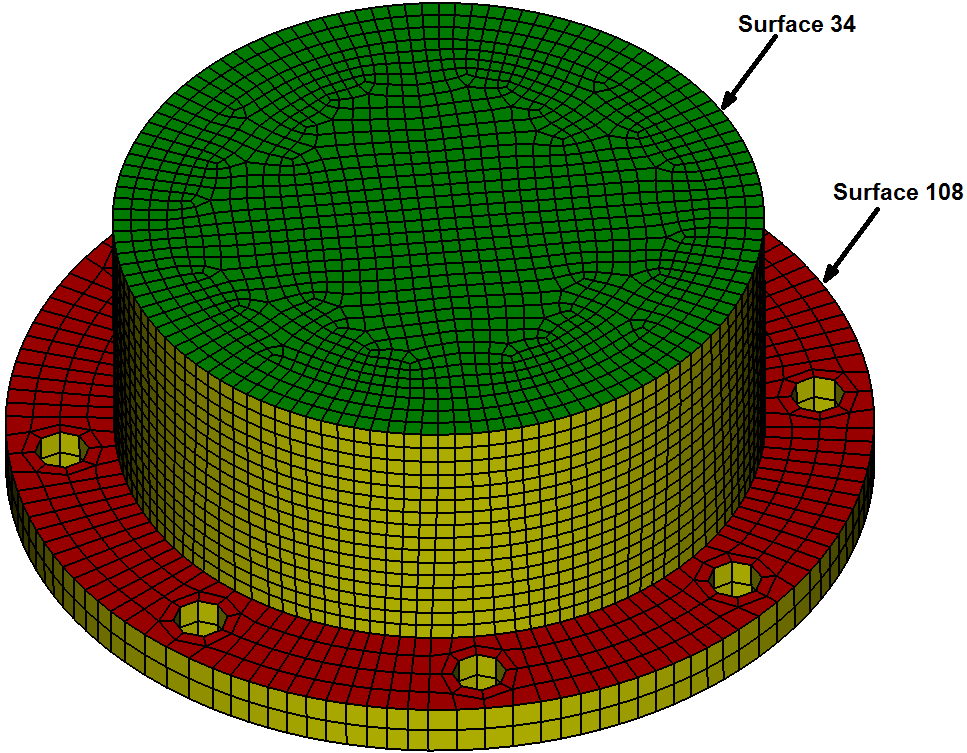
Figure 415: The mesh from Figure 414 scaled with the command "Scale Mesh Multi 2". The structured mesh on surface 108 is replaced with a paved mesh.
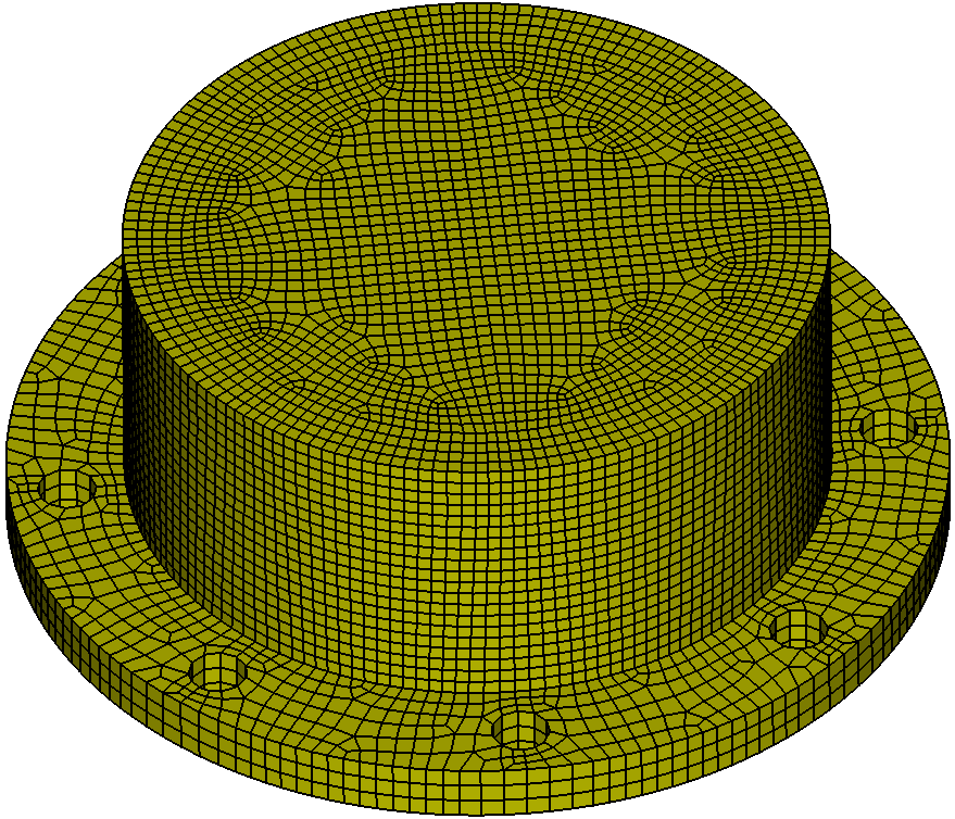
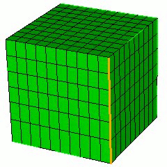
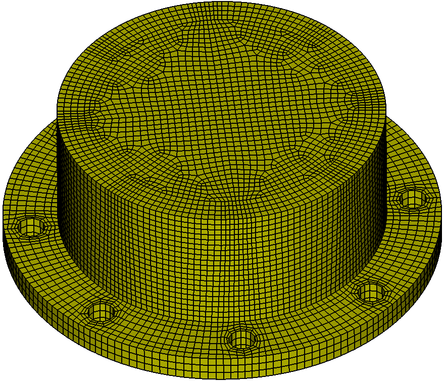
Figure 416: The mesh from Figure 412 scaled with the command "Scale Mesh Multi 2 force_structured in Surface 108". The structured mesh in surface 108 is maintained, while the remainder of the volume is scaled with swept blocks.
[thin_gap_intervals <value, default=2>]
[fix_all_gaps] [max_feature_length]
In general, maintain_structure should result in a smoother scaled mesh than the other algorithms, however, sometimes it can introduce some skew in the scaled elements. If skew is introduced by scaling using maintain_structure, try either increasing the thin_gap_intervals parameter, specifying fix_all_gaps, decreasing the max_feature_length parameter, or all three.
[feature_angle <value>]
[max_aspect_ratio <value> in volume <ids>]
[smooth_volume {ON|off}]
5.6.13 Node and Nodeset Repositioning
A capability to reposition nodesets and individual nodes is provided. This capability will retain all the current connectivity of the nodes involved, but it cannot guarantee that the new locations of the moved nodes do not form intersections with previously existing mesh or geometry. This capability is provided to allow the user maximum control over the mesh model being constructed, and by giving this control the user can possible create mesh that is self-intersecting. The user should be careful that the nodes being relocated will not form such intersections.
Nodeset <nodeset_list> Move <delta_x> <delta_y> <delta_z>
Individual nodes can be repositioned using the node move command. Moves are specified as relative displacements.
To move a node
On the Command Panel, click on Mesh and then Node.
Click on the Move Node action button.
Select Move XYZ from the drop-down menu.
Enter the appropriate value for Node ID(s). This can also be done using the Pick Widget function.
Enter the appropriate values for Delta X, Delta Y and Delta Z or manually move the node by dragging it to the desired location.
Click Apply.
Node <range> Move <delta_x> <delta_y> <delta_z>
Node <range> Move {[X <val>] [Y <val>] [Z <val>]}
On the Command Panel, click on Mesh and then Node.
Click on the Move Node action button.
Select Normal to Surface from the drop-down menu.
Enter the appropriate value for Node ID(s) and Surface ID. This can also be done using the Pick Widget function.
Enter the appropriate values for Distance.
Click Apply.
Node <range> Move Normal to Surface <id> distance <val>
Node <range> Move Location <options>
Node <range> Move Direction <options>
5.6.14 Mesh Pillowing
Figure 417: : A single hex before (a) and after (b) a pillow operation. The far right (c) depicts a pillow operation with the front surface designated as a 'through' surface.
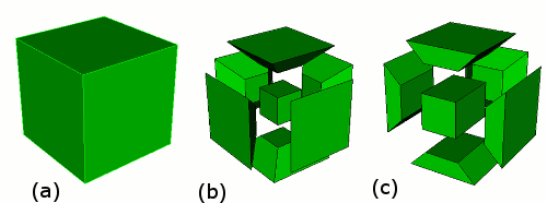
During a typical pillow operation, the user selects a set of elements, called a ’shrink set’, to define what elements will be operated on. All elements on the outer boundary of the shrink set are then shrunk towards the center of the set. New elements are then created to fill the gap between the original boundary and the shrunk boundary. The newly created elements form the pillow around the selected shrink set. Figure 417a and 1b show an example of a pillow operation performed on a single hex. Geometry surfaces, or mesh element faces can be specified as through surfaces for the pillowing operation. This means that the pillow will extend through the selected surfaces, and no new elements will be created along them. Figure 417c shows the effect of pillowing a single hex with one surface selected as a through surface.
In some cases a shrink set may not be valid due to the geometry of a specific region. As the exterior nodes of the shrink set move towards the middle they must be able to maintain appropriate geometric associations. Nodes on vertices must move along curves, nodes on curves must move along surfaces. If there are multiple curves or surfaces along which an exterior node might travel, then the ownership is ambiguous and the pillowing will fail.
Using the optional distance keyword with a specified value allows manual control of the distance that each boundary element is shrunk towards the center of the shrink set. If no distance value is specified, an appropriate value is calculated for each element. If a distance value is specified, all newly created nodes will have their position fixed by default. This allows the user to smooth the mesh without altering the node positions of the newly created hexes. If the optional unfix_nodes keyword is used, this default behavior is changed, and any smooth operations will alter the newly created node locations. By default, a smooth operation is automatically performed following any pillow operation unless the optional no_smooth keyword is used.
Similar analogous commands are available for creating a pillow around a set of two dimensional faces.
To use mesh pillowing
On the Command Panel, click on Mesh.
Click on Volume, Surface, Curve, Vertex, Hex or Quad.
Click on the Refine action button.
Select Pillowing from the drop-down menu.
Enter the appropriate value for the selected ID. This can also be done using the Pick Widget function.
Enter in any other appropriate settings.
Click Apply.
Pillow Hex <ids> [ Through { [Surface <ids>][Face <ids>][Tri <ids>] } ] [ Distance <value> ] [ Unfix_nodes ] [ No_smooth ]
Pillow Face <ids> [ Through Curve <ids> ] [ Distance <value> ] [ Unfix_nodes ] [No_smooth]
Figure 418: : Example model using pillow operations to create ordered nodes a specified distance around the boundary of a mesh.
5.6.15 Remeshing
Mesh generation is frequently an iterative process of meshing, deleting the mesh, and remeshing. The remesh command is a convenient tool to bypass the mesh deletion process when used to remesh a volume. You may also use the remesh command to replace a localized set of deformed tetrahedra after analysis. Thus, remeshing can become part of an optimization loop.
Remesh Volume <range>
To remesh tetrahedra
On the Command Panel, click on Mesh and then Tet.
Click on the Remesh action button.
Select Remesh Entities.
Select Tet(s), Volumes(s) or Block(s) and enter the appropriate value. This can also be done using the Pick Widget function.
Optionally, enter in any other appropriate settings.
Click Apply.
Remesh {Volume|Block|Tet} <range> [FIXED|free]
Remesh Tet <id_range> | [quality <tet_metric> [less than|greater than] <value> ...] [inflate <value>][FIXED|free][preview]
5.6.15.1 Remeshing a Swept Volume Mesh
The remesh command can be useful when using the sweep scheme. When a sweep scheme is applied to the volume, it will delete the target surface mesh on a volume with one of the sweeping schemes and then remesh the volume. It is useful when changing between sweep smooth options as in the following example below.
volume 1 scheme sweep
mesh volume 1
At this stage, the user may discover that poor quality elements may have been generated. The user could then do the following:
volume 1 sweep smooth winslow
remesh volume 1
At this point, the volume is remeshed using the sweep smooth winslow option.
5.6.15.2 Remeshing Tetrahedra
When used for tetrahedra, the remesh command generates a new tetrahedral mesh after deleting the existing mesh described by the list of tetrahedra, volumes, or blocks. When remeshing a list of tetrahedra, the smallest set of tets possible is replaced, which often means a partial remeshing of volumes, surfaces and/or curves. This set will always include the input list of tetrahedra but may include more.
Each tetrahedron may only be in one volume or block, but the list of tetrahedra may span volumes or blocks. Each block is treated individually if multiple blocks are specified.
The default FIXED option will ensure that any triangle or edge in the tetrahedron list to be remeshed that lie on geometric surfaces or curves will not be affected by the remesh operation. In contrast, the free option allows edges and triangles on curves and surfaces to be removed and remeshed. Use the FIXED option when it is important to maintain the boundary mesh configuration fixed, otherwise the free option will remesh the portions of curves and surfaces in the remesh region.
The remesh command can be used to selectively remove and remesh a small portion of tetrahedron in the mesh that have been identified as poor quality. This can be an effective tool for improving mesh quality on a deformed mesh following an analysis without the need to regenerate the full mesh.
The quality option will identify those tetrahedra from the full model and apply the remeshing opertaion only to those tetrahedra. Any of the standard quality metrics for tetrahedra may be used as the <tet_metric>. These include: aspect ratio bet, aspect ratio gam, element volume, condition no., jacobian, scaled jacobian, shape, relative size, shape and size, distortion, allmetrics, algebraic and traditional. The metric specification is used in conjunction with a less than or greater than specification and a threshold value. For example, the syntax below would remesh all tetrahedra in the mesh who’s scaled jacobian metric was less than 0.2.
remesh tet quality scaled jacobian less than 0.2 inflate 1 free
This command also allows for multiple quality criteria. For example, the following command would use both aspect ratio and scaled jacobian as criteria for remeshing. Any number of quality criteria may be included in the command syntax:
remesh tet quality scaled jacobian less than 0.2 quality aspect ratio bet greater than 4 inflate 1 free
Sizing functions may be used with tet remeshing. See Mesh Adaptivity and Sizing Functions and Exodus II-based Field Function for more information.
5.6.15.3 Inflating a set of Tets
Inflate [group <id>|tet <range>][manifold][layer <value>][add|create <"name">][draw]
group<id>|tet<range>: input to this command can be with a group name, group id, or a range of tets. The group must contain at least 1 tet. The tets need not be contiguous.
manifold: This option will add tets to the set where the boundary or skin of the tets meet at a single edge or node. This ensures that a complete valid manifold definition of the boundary of the set of tetrahedra can be defined. This is important for the tetrahedral mesh generator which requires a manifold boundary definition. both layer and manifold can be used in the same command.
layer <value>: This option will add the number of layers of tets indicated by value to the set. A layer is defined by all tets connected by at least a node to the skin of the existing set. This option alone does not guarantee a valid manifold definition. Use both the layer and manifold in the same command options to ensure a manifold definition.
add|create<"name">: The add option will add tets in the inflated region to the input group. An input group must be specified for this to be a valid option. The create option will create a new group and add all tets (including the input), to a new group specified by <"name">. If neither add nor create are specified, a new default group named "inflated_tets" will be created. If a group of that name already exists, it will be added to.
draw: The draw option will display both the input set of tets and the inflated tets in the graphics window. The input tets will be displayed in green and the inflated tets will be displayed in red.
Examples:
Generate a simple tet mesh. For tets with ids 1 to 10, define a 1 layer buffer and ensure it maintains a manifold boundary. The result will be placed in a new group called "inflated_tets" and displayed in the graphics window.
brick x 10
vol 1 scheme tetmesh
mesh vol 1
inflate tet 1 to 10 layer 1 manifold draw
Create a group called "bad_tets"containing all tets in volume 1with quality metric (scaled Jacobian) less than 0.2. Expand that group by one layer and remesh it.
group ’bad_tets’ equals qual vol 1 scaled high 0.2
inflate bad_tets layer 1 manifold add
remesh tet in bad_tets
5.6.16 Hexset Command
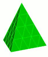
The hexset separate command is designed to create groups containing hexahedral elements based an enclosing set of triangles.
Hexset Hex <range> Separate Tri <range> [draw]
The inside and outside hex groups are separated into contiguous regions. Depending on the triangles used to intersect the hexes, there may be multiple inside and/or outside groups. In that case, the first inside group would be named "inside_hexes". The second would be named "inside_hexes@A" and so forth.
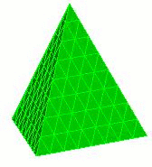
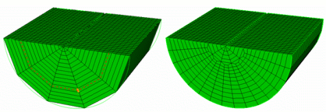
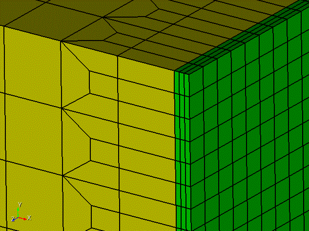
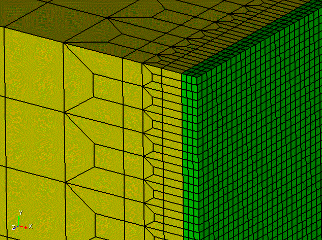
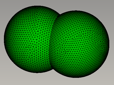
For example, given a tri-meshed volume as shown below:
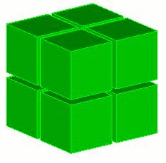
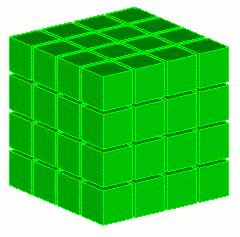
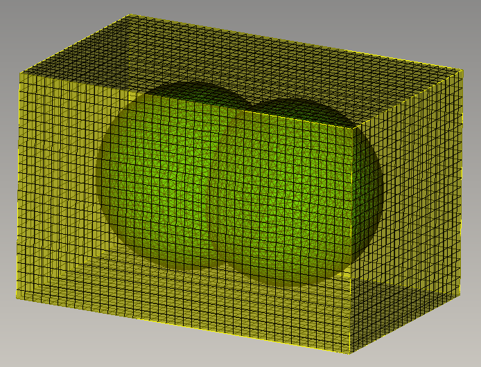
We create a bounding box and mesh it with hexes.
we issue the command, hexset hex all separate tri in surf 1 2, to get these results:
draw outside_hexes
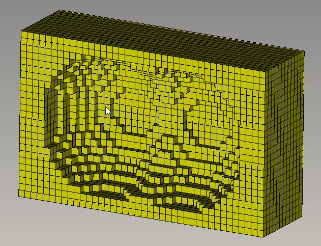
draw intersected_hexes
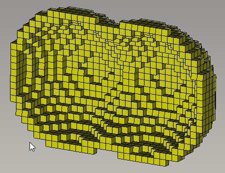
draw inside_hexes
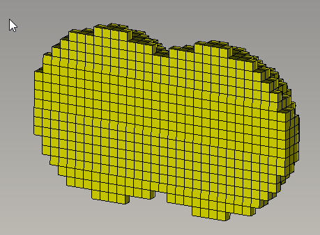
Combining all three images we see outside, intersecting and inside hexes.