5.4 Meshing Schemes
Meshing schemes in Cubit can be divided into four broad categories as detailed in the following sections.
If no scheme is selected, Cubit will attempt to assign a scheme using the automatic scheme selection methods.
5.4.1 Traditional Meshing Schemes
Traditional meshing schemes are used to apply a mesh to an existing geometry using the methods described in Meshing the Geometry (i.e. setting a scheme, applying interval sizes, and meshing). Traditional meshing schemes are available for all geometry types.
|
5.4.2 Free Meshing Schemes
Free meshing schemes will create a free-standing mesh without any prior existing geometry. The final mesh will have mesh-based geometry.
5.4.3 Conversional Meshing Schemes
Conversional meshing schemes are used to convert an existing mesh into a mesh of different element type or size. For example, the THex scheme will convert a tetrahedral mesh into a hexahedral mesh.
5.4.4 Duplication Meshing Schemes
Duplication meshing schemes are used to copy an existing mesh from one geometry onto another similar geometry.
5.4.5 Parallel Meshing Scheme
The Sculpt algorithm is an all-hex, automatic, parallel meshing scheme available in the Cubit Pro version.
5.4.6 General Meshing Information
Information on specific mesh schemes available in Cubit is given in this section. The following sections have important meshing-related information as well, and should be read before applying any of the mesh schemes described below.
In most cases, meshing a geometric entity in Cubit consists of three steps:
Set the interval number or size for the entity (See Interval Assignment.)
Set the scheme for the object, along with any scheme-specific information, using the scheme setting commands described below.
Mesh the object, using the command:
Mesh {geom_list}
After meshing is completed, the mesh quality is automatically checked (see Mesh Quality Assessment), then the mesh is drawn in the graphics window.
The following table classifies the meshing schemes with respect to their applicable geometry.
|
|
|
5.4.7 Automatic Scheme Selection
{geom_list} Scheme Auto
5.4.7.1 Default Scheme Selection
If the user does not set a scheme for a particular entity and chooses to mesh the entity, Cubit will automatically run the auto scheme selection algorithm and attempt to set a scheme. In cases where the auto scheme selection fails to choose a scheme, the meshing operation will fail. In this case explicit specification of the meshing scheme and/or further geometry decomposition may be necessary.
Set Default Element [Tet|Tri|HEX|QUAD|None]
Previous functionality of Cubit used a default scheme of map and interval of 1 for all surface and volume entities. For backwards compatibility and if this behavior is still desired, the none option may be used on the set default element command.
5.4.7.2 Auto Scheme Selection General Notes
In general, automatic scheme selection reduces the amount of user input. If the user knows the model consists of 2.5D meshable volumes, three commands to generate a mesh after importing or creating the model are needed.
To automatically calculate the meshing scheme
On the Command Panel, click on Mesh and then Volume.
Click on the Mesh action button.
Enter the appropriate value for Select Volumes. This can also be done using the Pick Widget function.
Select Automatically Calculate from the drop-down menu.
Click Apply Scheme then click Mesh.
volume all size <value>
volume all scheme auto
mesh volume all
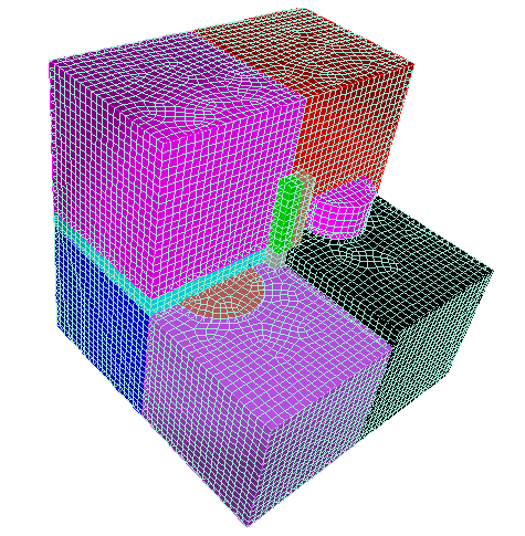
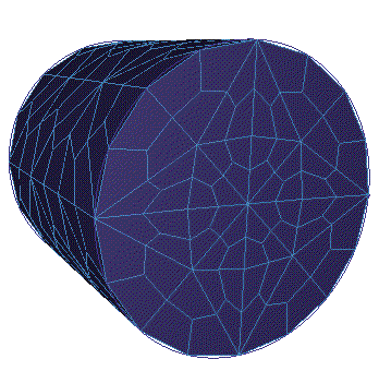
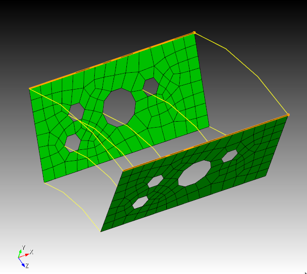
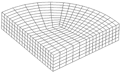
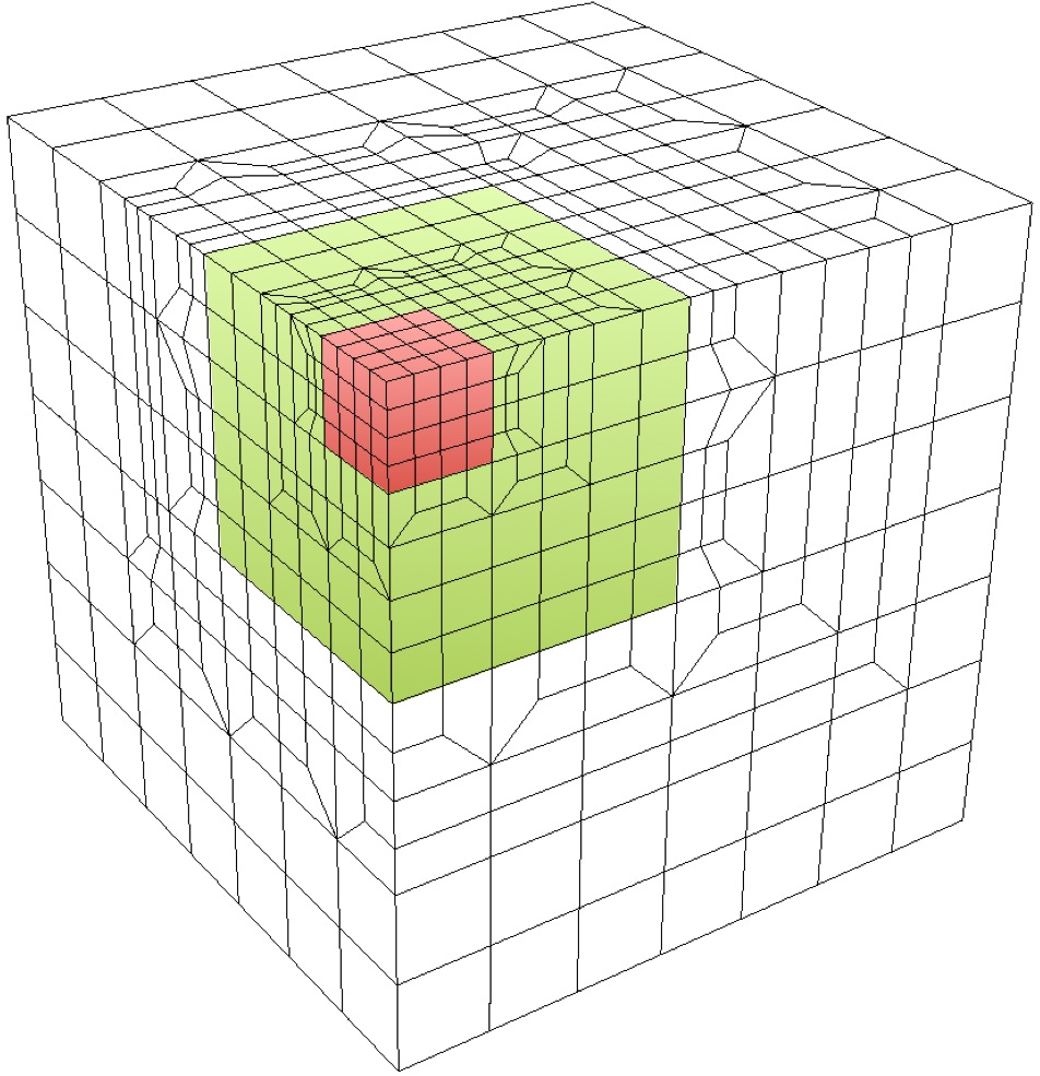
The model shown in the following figure was meshed using these three commands (part of the model is not shown to reveal the internal structure of the model).
Figure 227: Non-trivial model meshed using automatic scheme selection
5.4.7.3 Scheme Firmness
Meshing schemes may be selected through three different approaches. They are: default settings, automatic scheme selection, and user specification. These methods also affect the scheme firmness settings for surfaces and volumes. Scheme firmness is completely analogous to interval firmness.
{geom_list} Scheme {Default | Soft | Hard}
Scheme firmness settings can only be applied to surfaces and volumes.
This may be useful if the user is working on several different areas in the model. Once she/he is satisfied with an area’s scheme selection and doesn’t want it to change, the firmness command can be given to hard set the schemes in that area. Or, if some surfaces were hard set by the user, and the user now wants to set them through automatic scheme selection then she/he may change the surface’s scheme firmness to soft or default.
5.4.7.4 Surface Auto Scheme Selection
Surface auto scheme selection (White, 99) will choose between Pave, Submap, Triprimitive, and Map meshing schemes, and will always result in selecting a meshing scheme due to the existence of the paving algorithm, a general surface meshing tool (assuming the surface passes the even interval constraint).
[Set] Scheme Auto Fuzzy [Tolerance] {value} (value in degrees)
5.4.7.5 Volume Auto Scheme Selection
When automatic scheme selection is called for a volume, surface scheme selection is invoked on the surfaces of the given volume. Mesh density selections should also be specified before automatic volume scheme selection is invoked due to the relationship of surface and volume scheme assignment.
Volume scheme selection chooses between Map, Submap and Sweep meshing schemes. Other schemes can be assigned manually, either before or after the automatic scheme selection.
Volume scheme selection is limited to selecting schemes for 2.5D geometries, with additional tool limitations (e.g. Sweep can currently only sweep from several sources to a single target, not multiple targets); this is due to the lack of a completely automatic 3D hexahedral meshing algorithm. If volume scheme selection is unable to select a meshing scheme, the mesh scheme will remain as the default and a warning will be reported to the user.
Volume scheme selection can fail to select a meshing scheme for several reasons. First, the volume may not be mappable and not 2.5D; in this case, further decomposition of the model may be necessary. Second, volume scheme selection may fail due to improper surface scheme selection. Volume schemes such as Map, Submap, and Sweep require certain surface meshing schemes, as mentioned previously.
5.4.8 Conversion
5.4.8.1 HTet
Applies to: Volumes
Summary: Converts an existing hex mesh into a conforming tetrahedral mesh.
HTet Volume <range> {UNSTRUCTURED | structured}
Unlike other meshing schemes in this section, The HTet command requires an existing hexahedral mesh on which to operate. Rather than setting a meshing scheme for use with the mesh command, the HTet command works after an initial hex mesh has been generated.
Two methods for decomposing a hex mesh into tetrahedra are available. Set the method to be used with the optional arguments unstructured and structured. The unstructured method is the default. Figure 228 shows the difference between the two methods:
Figure 228: Left: Unstructured method creates 6 tets per hex. Right: Structured method creates 28 tets per hex
5.4.8.1.1 Unstructured
This method creates 6 tetrahedra for every hexahedra. No new nodes will be generated. The orientation of the 6 hexahedra will be based upon the element node numbering, as a result orientations may change if node numbering changes. This method is referred to as unstructured because the number of tetrahedra adjacent each node will be relatively arbitrary in the final mesh. Tetrahedral element quality is generally sufficient for most applications, however the user may want to verify quality before performing analysis.
5.4.8.1.2 Structured
With this approach, 28 tetrahedra are generated for every hexahedra in the mesh. This method adds a node to each face of the hex and one to the interior. Although this method generates significantly more elements, the orientation and quality of the resulting tetrahedra are more consistent. Each previously existing interior node in the mesh will have the same number of adjacent tetrahedra.
5.4.8.2 QTri
Applies to : Surfaces
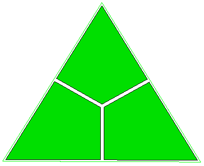
Summary: Meshes surfaces using a quadrilateral scheme, then converts the quadrilateral elements into triangles.
Surface <range> Scheme Qtri [Base Scheme quad_scheme>]
QTri {Surface <range> | Face <range> }
Set QTri Split [2|4]
Set QTri Test {Angle|Diagonal}
Discussion: QTri is used to mesh surfaces with triangular elements. The surface is, first, meshed with the quadrilateral scheme, and, then, the generated quads are split along a diagonal to produce triangles. The first command listed above sets the meshing scheme on a surface to QTri. The second form sets the scheme and generates the mesh in a single step.
In the first command, the user has the option of specifying the underlying quadrilateral meshing scheme using the base scheme <quad_scheme> option. If no base scheme is specified, Cubit will automatically select a scheme. For non-periodic surfaces, the base scheme will be set to scheme pave. For periodic surfaces, the base scheme will be set to scheme map.
Generally, the second command, Qtri Surface <range>, is used on surfaces that have already been meshed with quadrilaterals. If, however, this command is used on a surface that has not been meshed, a base scheme will automatically be selected using CUBIT’s auto-scheme capabilities. The user can over-ride this selection by specifying a quadrilateral meshing scheme prior to using the qtri command (using the Surface <range> Scheme <quad_scheme> command). QTri may also be performed on quadrilateral elements on a surface or a subset of quadrilateral elements on a surface. to split existing quadrilaterals the QTri command can be given a list of faces.
In addition to the default 2 tris per quad, the set qtri split command may alter the QTri scheme so that it will split the quad into 4 triangles per quad. Where the 4 option is used, an additional mesh node is placed at the centroid of each quad.
There are two methods that may be used to calculate the best diagonal to use for splitting the quadrilateral elements: angle or diagonal. The angle measurement uses the largest angle, while the diagonal option uses the shortest diagonal. The largest angle measurement will be more accurate but takes more time.
Also, the QTri scheme is used in the TriMesh command as a backup to the TriAdvance triangle meshing scheme.
5.4.8.3 THex
Applies to: Volumes
Summary: Converts a tetrahedral mesh into a hexahedral mesh.
THex Volume <range>
Discussion: The THex command splits each tetrahedral element in a volume into four hexahedral elements, as shown in Figure 230. This is done by splitting each edge and face at its midpoint, and then forming connections to the center of the tet.
When THexing merged volumes, all of the volumes must be THexed at the same time, in a single command. Otherwise, meshes on shared surfaces will be invalid. An example of the THex algorithm is shown in Figure 231.
Figure 230: Conversion of a tetrahedron to four hexahedra, as performed by the THex algorithm.
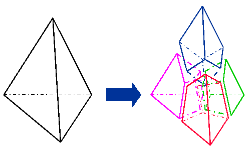
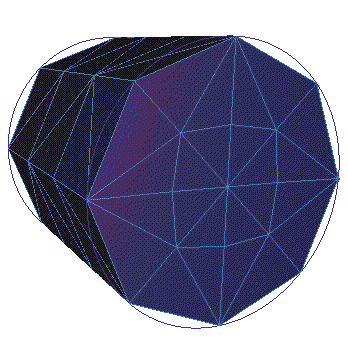
Figure 231: A cylinder before and after the THex algorithm is applied.
5.4.8.4 TQuad
Applies to: Surfaces
Summary: Converts a triangular surface mesh into a quadrilateral mesh.
TQuad Surface <range>
Discussion: The TQuad command splits each triangular surface element in four quadrilateral elements, as shown in Figure 232. This is done by splitting each edge at its midpoint, and then forming connections to the center of the triangle. The result is the same as using the THex algorithm, but only applies to surfaces. In general it is better to use a mapped or paved mesh to generate quadrilateral surface meshes. However, the TQuad scheme may be useful for converting facet-based triangular meshes to quadrilateral meshes when remeshing is not possible.
Figure 232: A triangle split into 3 quads using the TQuad scheme
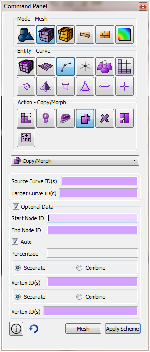
5.4.9 Copying a Mesh
Applies to: Curves, Surfaces, Volumes
Summary: Copies the mesh from one entity to another
To copy a mesh on a curve
On the Command Panel, click on Mesh and then Curve.
Click on the Copy/Morph action button.
Enter the values for Source Curve ID(s) and Target Curve ID(s). This can also be done using the Pick Widget function.
Optionally, click on Optional Data to further specify the settings.
Click on Appy Scheme and then Mesh.
The Command Panel GUI is shown below:
Curve <range> Scheme Copy source Curve <range> [Source Percent [<percentage> | auto]] [Source [combine|SEPARATE]] [Target [combine|SEPARATE]] [Source Vertex <id_range>] [Target Vertex <id_range>]]
Copy Mesh Curve <curve_id> Onto Curve <curve_id_range> [Source Node <starting node id> <ending node id>] [Source Percent [<percentage>|auto]] [Source Vertex <id_range>] [Target Vertex <id_range>]
To copy a mesh on a surface
On the Command Panel, click on Mesh and then Surface.
Click on the Copy/Morph action button.
Using the pickwidgets in the command panel select source and target data.
To force copying of interior vertex loops select the "Interior Vertices" tab and enter in pairs of vertices to be matched when copying.
The Command Panel GUI is shown below:
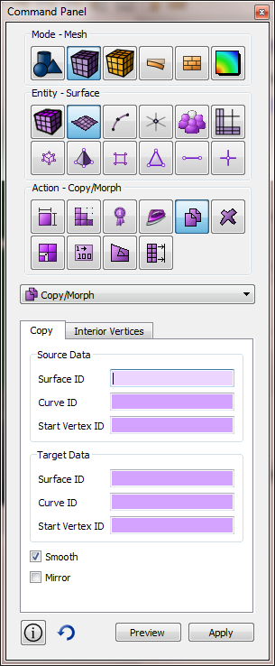
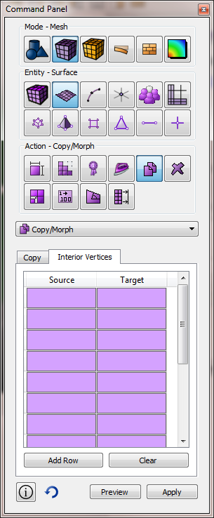
Copy Mesh Surface <surface_id> Onto Surface <surface_id> Source Curve<id> Target Curve <id> Source Vertex <id>Target Vertex <id> [Interior (pair vertex <id><id>)...] [smooth] [mirror] [preview]
Surface <id> Scheme copy source surface <id> source curve <id> target curve <id> source vertex <id> target vertex <id> [nosmoothing][mirror]
To copy a mesh on a volume
On the Command Panel, click on Mesh and then Volume.
Click on the Copy/Morph action button.
Enter the values for Source Volume ID(s) and Target Volume ID(s). This can also be done using the Pick Widget function.
Optionally, click on Optional Data to further specify the settings.
Click on Appy Scheme and then Mesh.
The Command Panel GUI is shown below:
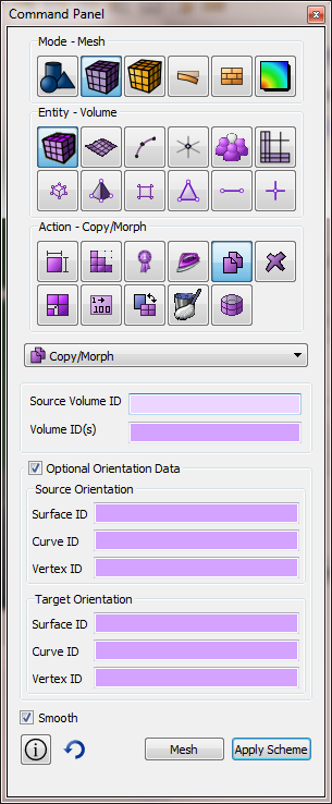
Volume <range> Scheme Copy [Source Volume] <id> [[Source Surface <id> Target Surface <id>] [Source Curve <id> Target Curve <id>] [Source Vertex <id> Target Vertex <id>]][Nosmoothing]
Copy Mesh Volume <volume_id> Onto Volume <volume_id> [Source Vertex <vertex_id> Target Vertex <vertex_id>] [Source Curve <curve_id> Target Curve <curve_id>] [Nosmoothing]
Set Morph Smooth {on | off}
Discussion: If the user desires to copy the mesh from a surface, volume, curve, or set of curves that has already been meshed, the copy mesh scheme can be used. Note that this scheme can be set before the source entity has been meshed; the source entity will be meshed automatically, if necessary, before the mesh is copied to the target entity. The user has the option of providing orientation data to specify how to orient the source mesh on the target entity. For example, when copying a curve mesh, the user can specify which vertex on the source (the source vertex) gets copied to which vertex on the target (the target vertex). If you need to reference mesh entities for the copy, use the copy mesh commands. If no orientation data is specified, or if the data is insufficient to completely determine the orientation on the target entity, the copy algorithm will attempt to determine the remaining orientation data automatically. If conflicting, or inappropriate, orientation data is given, the algorithm attempts to discard enough information to arrive at a proper mesh orientation.
Curve mesh copying has certain options that allow the copying of just a section of the source curves’ mesh. These options are accessed through the extra keyword options. The percent option allows the user to specify that a certain percentage of the source mesh be copied–in this context the auto keyword means that the percentage will be calculated based on the ratio of lengths of the source and target curves. The combine and separate keywords relate to how the command line options are interpreted. If the user wishes to specify a group of target curves that will each receive an identical copy of a source mesh, then the target separate option should be used (this is the default). If, however, the user wishes the source mesh to be spread out along the range of target curves, then the target combine option should be used. The source curves are treated in a similar fashion.
Surface mesh copying with multiple holes in the surface may require matching up interior pair vertices. This will be required if the algorithm cannot match them up spatially. Interior pair vertices can be specified with the option interior pair vertex ...
Volume mesh copying depends on the surface copying scheme. Because of this, the target volume must not have any of its surfaces meshed already.
copy mesh surf 23 onto surf 14 source curve 1 source vertex 1 target curve 24 target vertex 20
5.4.10 Radialmesh
Creates a free cylindrical mesh with precise node locations based on input radii, angles, and offsets, then creates mesh-based geometry to fit the mesh.
Create Radialmesh \
NumZ <val> [Span <val>] \
Zblock 1 [<offset val>] \
{Interval|Bias|Fraction|First Size} <val> \
[{Interval|Bias|Fraction|Last Size} <val>] \
Zblock 2 [<offset val>] \
{Interval|Bias|Fraction|First Size} <val> \
[{Interval|Bias|Fraction|Last Size} <val>] \
... NumZ \
NumR <val> {Trisection|Initial Radius<val>} \
Rblock 1 <offset radius val> \
{Interval|Bias|Fraction|First Size} <val> \
[{Interval|Bias|Fraction|Last Size} <val>] \
Rblock 2 <offset radius val> \
{Interval|Bias|Fraction|First Size} <val> \
[{Interval|Bias|Fraction|Last Size} <val>] \
... NumR \
NumA <val> [Full360] [Span <val>] \
Ablock 1 [<offset angle val>] \
{Interval|Bias|Fraction|First Angle} <val> \
[{Interval|Bias|Fraction|Last Angle} <val>] \
Ablock 2 [<offset angle val>] \
{Interval|Bias|Fraction|First Angle} <val> \
[{Interval|Bias|Fraction|Last Angle} <val>] \
... NumA
The purpose of the radialmesh command is to create a cylindrical mesh with precise node locations. Unlike all other meshing commands which place nodes using smoothing algorithms to optimize element quality, node locations for the radialmesh command are calculated based on the input radii, angles, and offsets. In addition, the radialmesh command does not mesh existing geometry. Rather, it creates a mesh based on the input parameters, after which a mesh-based geometry is created to fit the free mesh.
The radialmesh command requires input for the 3 coordinate directions (Z, radial, angular). The number of blocks in each direction is specified with the numZ, numR, and numA values in the command. Each block forms a new volume in the final mesh. All bodies in the mesh are merged to form a conformal mesh between blocks.
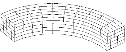
The Radialmesh command can create meshes which span any angle greater than 0.0 up to 360 degrees. In addition, meshes can model either a tri-section (see Figure 237), or a non-trisection mesh (see Figure 238).
create radialmesh \
numZ 1 zblock 1 1 interval 5 \
numR 3 trisection rblock 1 2 interval 5 \
rblock 2 3 interval 5 \
rblock 3 4 interval 5 \
numA 1 span 90 ablock 1 interval 10
The command to generate the mesh in Figure 238 is:
create radialmesh \
numZ 1 zblock 1 1 interval 5 \
numR 1 initial radius 3 rblock 1 4 interval 5 \
numA 1 span 90 ablock 1 interval 10
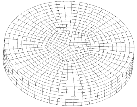
A mesh can span an entire 360 degrees by using the "full360" keyword. For example, the mesh in Figure 3 was generated with the following command:
create radialmesh numZ 1 zblock 1 1 interval 5 \
numR 3 trisection rblock 1 1 interval 5 \
rblock 2 2 interval 5 \
rblock 3 3 interval 5 \
numA 5 full360 span ablock 1 interval 5 \
ablock 2 interval 5 \
ablock 3 interval 5 \
ablock 4 interval 5
The user can control the number of intervals and the spacing of these intervals using the optional parameters in each rblock, zblock and ablock. There are 11 combinations that these can be combined as listed below:
Interval Only- Example: "interval 5." The block will be meshed with 5 equally spaced intervals.
First Size Only- Example: "first size 2.5." The block will be meshed with intervals of approximately 2.5 in length. The total number of intervals is internally calculated and depends on the overall block length.
Fraction Only- Example: "fraction 0.3333." The block will be meshed with intervals approximately 0.3333*overall block length.
Interval and Bias- Example: "interval 5 bias 1.5." There will be 5 intervals on the block, which each interval being 1.5 times the previous one. The length of each interval is calculated internally.
Interval and Fraction- Example: "interval 5 fraction 0.25." There will be 5 intervals on the block, the first being .25 of the length of the block with the remaining decreasing in size.
Interval and First Size- Example: "interval 5 first size 0.2." There will be 5 intervals on the block, the first being 0.2 in length. The remaining intervals will increase or decrease to fill the blocks length.
First Size and Last Size- Example: "first size 0.2 last size 0.4." The first interval will be 0.2 in length. The last interval will be 0.4 in length. The total number of intervals is internally calculated to allow for transition between the 2 specified sizes.
First Size and Bias- Example "first size 0.2 bias 0.85." The first interval will be 0.2 in length and the remaining intervals will scale by a factor of 0.85 from one to the next until the block is filled. The total number of intervals is internally calculated and depends on the overall block length.
Fraction and Bias- Example "fraction 0.25 bias 1.25." The first interval will be 0.25 of the overall block length and the remaining intervals will scale by a factor of 1.25 from one to the next until the block is filled. The total number of intervals is internally calculated and depends on the overall block length.
Interval and Last Size- Example: "last size 1.5 interval 5." The last interval will be 1.5 in length. The remaining intervals will scale up or down to fit 5 intervals in the block.
Last Size and Bias- Example: "last size 2.0 bias 1.1." The last interval will be 2.0 in length. The remaining intervals will scale by 1.1 until the block is filled. The total number of intervals is internally calculated and depends on the overall block length.
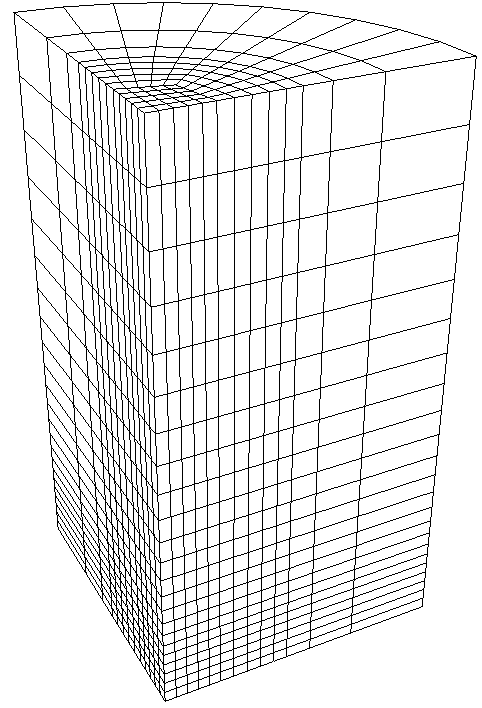
Figure 240 shows an example of a bias spaced mesh with the following command:
create radialmesh numZ 2 zblock 1 1 first size 0.2 \
zblock 2 10 first size 0.2 last size 1.0 \
numR 3 trisection rblock 1 1 interval 5 \
rblock 2 2 first size .25 \
rblock 3 5 first size .25 bias 2.0 \
numA 1 span 90 ablock 1 interval 5
5.4.11 Parallel Meshing
Cubit has been designed as a serial application, using a single CPU to generate its meshes. In some cases, where memory or time constraints are critical, parallel meshing may be necessary. Cubit currently provides a separate application designed to run in parallel either on a desktop or on massively parallel cluster machines. In these cases, Cubit can be used as a pre-processor to manipulate geometry and set up for meshing, however the actual meshing procedure is performed as a separate process or on another machine.
5.4.11.1 Sculpt
Sculpt is a separate parallel application designed to generate all-hex meshes on complex geometries with little or no user interaction. Sculpt was developed as a separate application so that it can be run independently from Cubit on high performance computing platforms. It was also designed as a separable software library so it can be easily integrated as an in-situ meshing solution within other codes. Cubit provides a front end command line and GUI for the Sculpt application. The command will build the appropriate input files based on the current geometry and can also automatically invoke Sculpt to generate the mesh and bring the mesh back to Cubit.
5.4.11.1.1 Preparing to Use Sculpt
5.4.11.1.1.1 Platforms
Sculpt is available for Windows, Mac and Linux operating systems.
5.4.11.1.1.2 Sculpt Installation
Sculpt is a stand-alone executable, separate from Cubit. In order for Cubit to start up Sculpt, it must be on your system and accessible to Cubit. The default installation of Cubit should install files in the correct locations for this to occur. Check with Cubit support if it did not come with your installation or you are not able to locate it or any of its supporting applications.
To run Sculpt from Cubit, four executable files are needed:
sculpt: Application that controls start-up of mpiexec and psculpt. Main entry point from Cubit, that checks for the existence and compatibility of either the system mpiexec application or will use a local cubit instalation of mpiexec.
psculpt: The main mpi-based Sculpt application. Requires mpiexec to run.
mpiexec: Standard application available on most linux-based operating systems for starting up mpi-based applications on multiple processors. This should be available with your Cubit installation, but is also available from http://open-mpi.org
epu: Used for combining multiple exodus files, generated with Sculpt, into a single exodus file. This executable is optional, but is useful for importing the resulting mesh into Cubit for viewing. It is part of the SEACAS tool suite developed by Sandia National Laboratories and is also included with your Cubit installation. It can also be obtained in open source form from https://github.com/gsjaardema/seacas.
Sculpt Parallel Path List |
See the Sculpt Parallel Path Command for more info on setting and customizing these paths.
The following image illustrates the process flow when the sculpt parallel command is used in Cubit.
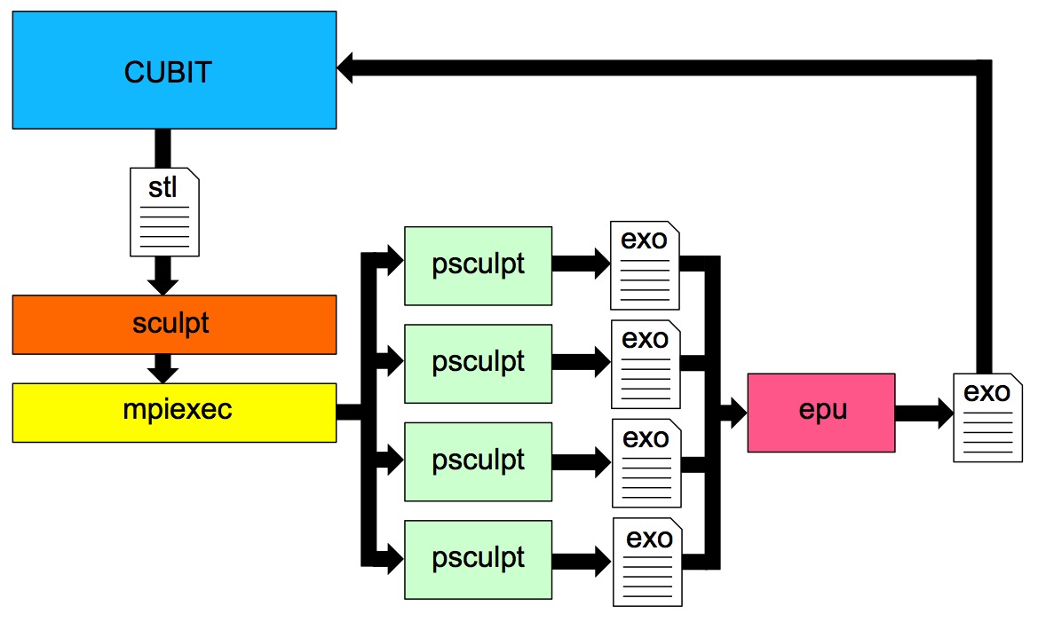
5.4.11.1.1.3 Sculpt Process Flow
For the Sculpt meshing process, a set of files, including a facet-based stl file are written to disk. The sculpt application is then started up which in turn invokes mpiexec to start up multiple instances of psculpt in parallel. psculpt then performs the meshing and writes one exodus file per processor. These files can then be combined using epu and then imported back into Cubit for viewing.
5.4.11.1.1.4 Setting your Working Directory
When using the Sculpt Parallel command in Cubit, several temporary files will be written to the current working directory. Because of this, it is important to set your working directory before using Sculpt to a desired location where you want these files placed.
5.4.11.1.2 Sculpt Parallel Command
The command syntax for preparing a model for Sculpt is:
Sculpt Parallel |
|
|
[size <value>|autosize <value>] |
The following table is a summary of options that can be invoked from the Cubit sculpt parallel command. It includes an abbreviated description of the option as well as the option’s default. If the option is not explicitly used in the command, the default value listed will be used. The Sculpt option is the corresponding command that can be used in a sculpt input file when sculpt is invoked directly from a terminal window. See Sculpt Application for more information.
Cubit Option |
| Description |
| Default |
| Sculpt Option |
|
|
|
|
| ||
|
|
|
|
| ||
|
|
|
|
| ||
|
|
|
|
| ||
|
|
|
|
| ||
|
|
|
|
| ||
|
|
|
|
| ||
|
|
|
|
| ||
|
|
|
|
| ||
|
|
|
|
| ||
|
|
|
|
| ||
|
|
|
|
| ||
|
|
|
|
| ||
|
|
|
|
| ||
|
|
|
|
| ||
|
|
|
|
| ||
|
|
|
|
| ||
|
|
|
|
| ||
|
|
|
|
| ||
|
|
|
|
| ||
|
|
|
|
| ||
|
|
|
|
| ||
|
|
|
|
| ||
|
|
|
|
| ||
|
|
|
|
| ||
|
|
|
|
| ||
|
|
|
|
| ||
|
|
|
|
| ||
|
|
|
|
| ||
|
|
|
|
| ||
|
|
|
|
| ||
|
|
|
|
| ||
|
|
|
|
| ||
|
|
|
|
| ||
|
|
|
|
| ||
|
|
|
|
| ||
|
|
|
|
| ||
|
|
|
|
| ||
|
|
|
|
| ||
|
|
|
|
|
5.4.11.1.3 Controlling the Execution of Sculpt
The following command options can be used to control the execution of Sculpt from within Cubit and can be used with the sculpt parallel command. Follow the links above for others not lsted here.
volume <ids> | block <ids> List of volumes or blocks to include in the mesh. One file containing a faceted representation (STL) per volume will be generated and saved in the current working directory to be used as input to Sculpt. Each volume will be treated as a separate material within sculpt and a conforming mesh will be generated where volumes touch. If the Block command is used, one file per block will be used. Each block represents a separate material in Sculpt.
fileroot ’<root filename>’ Root of file names for output. When the sculpt parallel command is executed, Cubit will generate multiple files in the working directory used for input to the Sculpt application. The ’<root filename>’ will be used as the basis for naming these files.
OVERWRITE | no_overwrite By default, Cubit will overwrite an existing set of files with the same ’<root filename>’. To over-ride, use the no_overwrite option.
absolute_path By default, Cubit will write the relative path names of files used in the .run and .diatom files. To force absolute path names to be written, use the absolute_path option.
EXECUTE | no_execute By default, Cubit will attempt to run sculpt in parallel on the machine Cubit is currently running on. To generate just the required input to run Sculpt at a later time or on another machine, use this option. A file of the form <root filename>.run will be generated in the current working directory. (for example "model.run"). Executing the .run file from the linux command line should run sculpt in parallel. It can also be used to run sculpt on a cluster where a Cubit executable may not be available.
size <value> | autosize <value> The size option is the absolute cell size for the Cartesian grid and is the same as the cell_size option in sculpt. The autosize option is a value between 0 and 10. It represents a model independent size where 1 is the small size and 10 is large. This is the same scaling factor used in Cubit’s auto sizing but is divided by ten. A size value will be computed from the selected autosize and used as the absolute cell size for the base Cartesian grid.
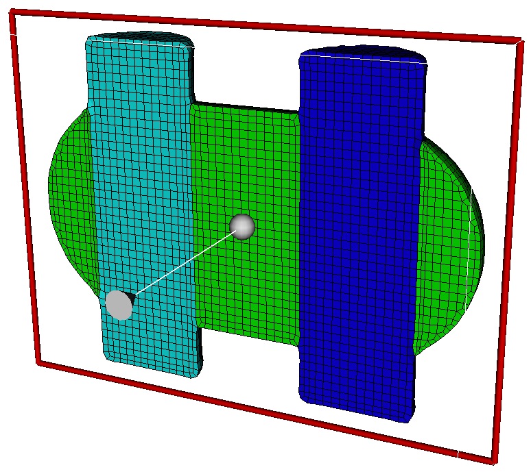
box location <options> location options define the bounds of the Cartesian grid. The first Location <option> defines the minimum Cartesian coordinate of the grid and the second, the maximum. The <options> can be any valid method for defining a coordinate location in cubit. In most cases the position option can be used. The default is computed as an enclosing bounding box with 2.5 additional cells on each side.
COMBINE | no_combine If the no_combine option is used, following execution of Sculpt, the resulting exodus meshes will not be combined using the epu seacas tool. Otherwise the default will automatically combine the meshes generated by each processor into a single mesh. Note that epu should be installed on your system and the path to epu defined using the sculpt parallel path command. Epu is a code developed by Sandia National Laboratories and is part of the SEACAS tool suite. It combines multiple Exodus databases produced by a parallel application into a single Exodus database. The epu program should be included with distributions of Cubit beginning with Version 15.0.
IMPORT | no_import If the no_import option is used, following execution of Sculpt, the result will be not be imported into Cubit as a free mesh. The default IMPORT option will automatically import the mesh that was generated in Sculpt. If the no_combine option has been used, then multiple free meshes will be imported with duplicate nodes and faces at processor domain boundaries. Otherwise a single free mesh, the result of the epu code, will be imported. Note that the resulting mesh will not be associated with the original geometry, however Block (material) definitions will be maintained. In addition, a separate group will be generated for each imported mesh (One per processor). The default will automatically import the mesh following mesh generation in Sculpt.
SHOW | no_show If the no_show option is used, while the external Sculpt process is running, no ouput from the Sculpt application will be displayed to the command window. Otherwise, the default SHOW is used and output from the Sculpt application will be echoed to the Cubit command window. This option is only effective if the no_execute is not used.
CLEAN | no_clean If the clean option is used, temporary files generated during the sculpt parallel command will be deleted. This includes any exodus mesh files, .stl, .diatom, .log and .run files. The default for this option is CLEAN, therefore, use the no_clean option to keep any temporary files generated as part of the current Sculpt run.
gen_input_file <file name> | no_gen_input_file An input file with the given file name will be generated when the command is executed. This is a text file containing all sculpt options used in the command. The input file is intended to be used for batch execution of sculpt. To run sculpt from the operating system command line you would use the -i option. For example: sculpt -i myinputfile.i -j 4 where myinputfile.i is the name of the input file specified with the gen_input_file option and -j 4 is the number of processors to use.
debug <value> The debug option is used only as a developer debugging tool. It will set the debug processor and sleep upon execution to allow a debugger to be attached to the process.
5.4.11.1.4 Sculpt Parallel Path Command
Sculpt Parallel Path [List|Psculpt|Epu|Mpiexec] |
list |
5.4.11.1.5 Sculpt Mesh Quality Control
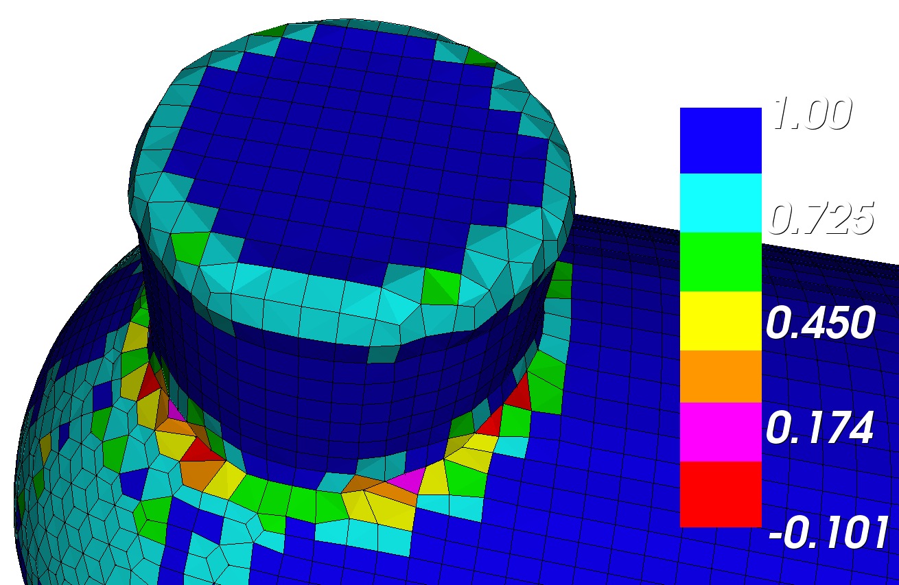
In most cases, the Sculpt tool can be used without adjusting default values. Depending on the characteristics of the geometry to be meshed, the default values may not yield adequate mesh quality. Upon completion, Sculpt reports to the command line, a summary of the mesh that was generated. This includes a summary of the mesh quality. Care should be taken to review this summary to ensure the minimum mesh quality is in a range suitable for analysis.
The element metric used for computing mesh quality in Sculpt is the Scaled Jacobian. This is a value between -1 and 1 that is a relative measure of the angles at the element’s nodes. A value of 1 indicates a perfect 90 degree angle between each of its edges. In most cases a value less than zero, or negtive Jacobian element, indicates an unusable mesh. Sculpt’s default settings try to achieve a minimum Scaled Jacobian of 0.2, which is normally usable in most analysis. The following discussion provides several options for adjusting the model or Sculpt parameters to help improve mesh quality.
- Locating poor mesh quality: When the Sculpt mesh has been imported back into CUBIT it is a good idea to display the element quality. You can do this with variations of the following commands:
quality hex all scaled jacobian
quality hex all draw mesh Identify regions where hexes are poor quality and zoom in to these regions.
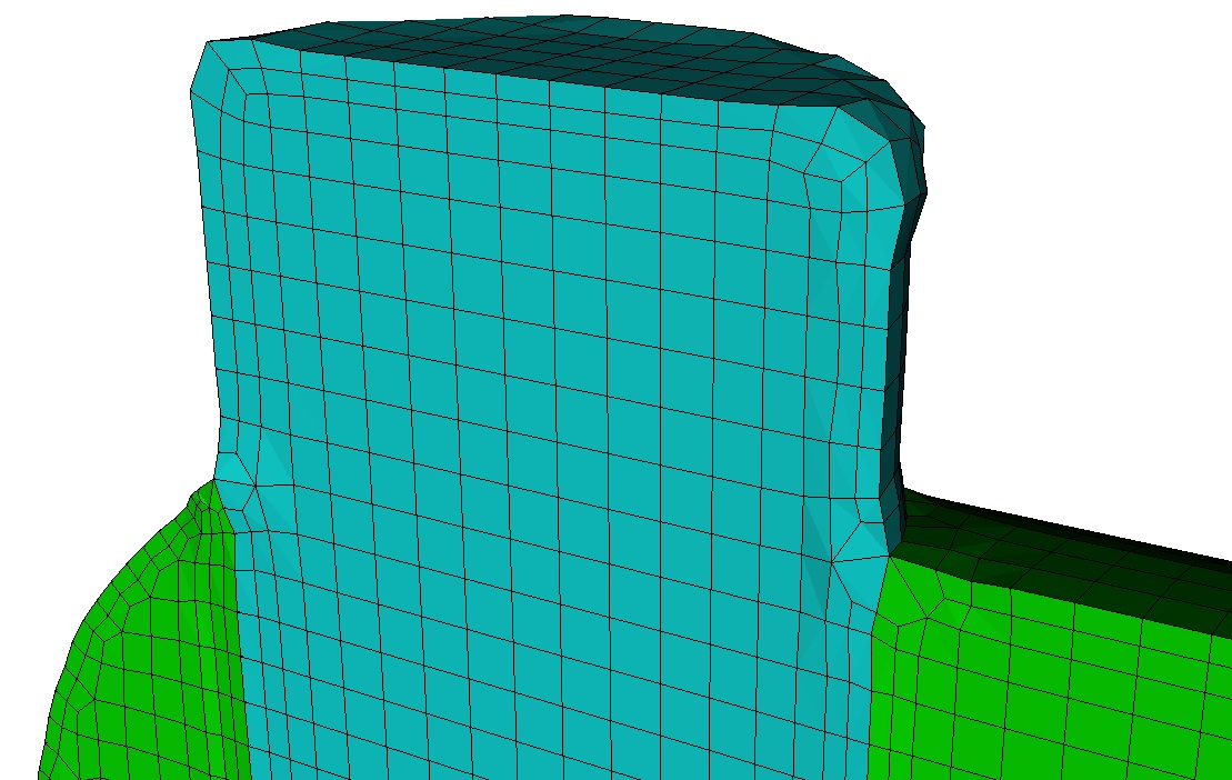
Modifying the geometry: Zooming in to poor quality elements may reveal that the mesh does not adequately represent the underlying geometry. In some cases you may find that small features, or small gaps between parts may be on the order of the size of the Sculpt cell size. If these features are not important to the analysis, you may consider using Cubit’s geometry modification tools to remove features or close small gaps.
Modifying the cell size: In cases where small geometric features or gaps are important to the simulation, it may be necessary to use a smaller base cell size. Use the size or autosize input parameters or increase the numbers of intervals. Normally to adequately capture a feature you would want the cell size to be no greater than about 1/3 to 1/2 the size of the smallest feature you would want to represent in the simulation.
Turning on Pillowing for multiple materials: For models that have more than one material that share an interface, unless the geometry is precisely aligned with the global axis, it is usually a good idea to turn on pillowing. Pillowing automatically inserts an additional layer of hexes at interface boundaries to improve mesh quality. Without pillowing may notice inverted or poor quality elements at curve interfaces where 2 or more materials meet.
- Modifying smoothing parameters: Sculpt includes a tiered approach to smoothing to improve element quality. It starts by applying smoothing to all nodes in the mesh and progressively restricts the smoothing operations to only those nodes that fall below a user-defined scaled Jacobian threshold. Default numbers of iterations and thresholds for each smoothing phase have been tuned for general use, however it may be worthwhile to adjust these parameters. The three smoothing phases include: Observing the mesh quality output to the command line following each smoothing iteration can provide some insight on the effect of modifying smoothing parameters.
Laplacian Smoothing: Applied to all elements. Very inexpensive fast approach to improve quality, but can result in degraded element quality if applied to excess. A fixed default of 2 iterations is applied to all hexes. Increasing the num_laplace parameter can improve some cases, especially convex shapes
Optimization Smoothing: Applied only to elements who’s scaled Jacobian falls below the opt_threshold parameter (default 0.6) and their surrounding elements. This approach uses a more expensive optimization technique to improve regions of elements simultaneously. The max_opt_iters parameter can control the maximum number of iterations applied (default is 5). Iterations will terminate, however, if no further improvement is detected. Because this method optimizes node locations simultaneously, neighboring nodes with competing optimum can sometimes limit mesh quality.
Spot Optimization: Also known as parallel coloring, is applied only to elements who’s element quality falls below the pcol_threshold parameter (default 0.2). This technique is the most expensive of the techniques, but focusses only on nodes that are immediately adjacent to poor quality hexes. Each node is smoothed independently of its neighbors, and may require a high number of iterations using the max_pcol_iters to achieve desired results. Increasing the pcol_threshold and max_pcol_iters may yield improved results.
Creating degenerate hexes: Some geometries will not permit a usable mesh with a traditional all-hex mesh. Sculpt includes the option to automatically and selectively collapse element edges to improve low-quality elements. The max_deg_iters and the deg_threshold values are used to control the creation of degenerates. Degenerate elements are treated as standard hex elements, but use repeated nodes in the eight-node connectivity array.
Creating hex-dominant mesh Another option for avoiding mesh quality issues is to generate a few tet elements in the mesh using the htet option. With this option you can specify a scaled Jacobian threshold value below which hexes will be converted to tet elements. The interface between hex and tet elements is managed by an automatically defined set of nodesets and sidesets that describe where multi-point constraints will be applied.
Defeaturing The defeature option does an initial filter on the cells of the base grid and attempts to reassign the material ID for cells that meet certain criteria. These are cases where a small grouping of cells form a small volume, or where protrusions exist that would otherwise be difficult or impossible to mesh with good quality elements. By reassigning the cells in these locations, in many cases it will allow the mesh to be acceptable. This operation may result in small changes to the boundary or surface definitions, however usually small enough to still be a reasonable approximation.
5.4.11.1.6 Sculpt Examples
sphere rad 1 |
5.4.11.1.6.1 Basic Sculpt
sculpt parallel |
5.4.11.1.6.2 Size and Bounding Box
delete mesh |
5.4.11.1.6.3 Meshing the Void
delete mesh |
5.4.11.1.6.4 Automatic Sideset Definition
In this example we illustrate the use of the sideset option.
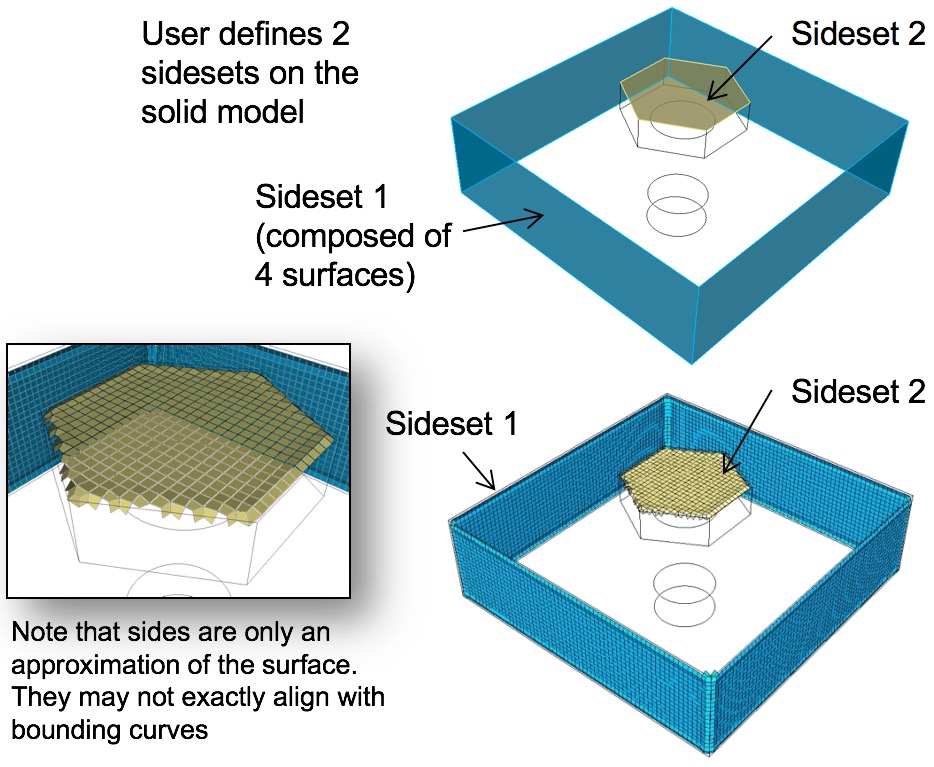
Generating sidesets on the free mesh with Cubit: Sideset boundary conditions can be manually created on the resulting free mesh from Sculpt using the standard sideset <sideset_id> face <id_range> syntax. The group seed command is also useful in grouping faces based on a feature angle to be used in a single sideset.
delete mesh |
Interfaces between materials
Exterior surfaces
Surfaces at the domain boundary
See the sideset option above for a description of other options for generating sidesets in Sculpt.
5.4.11.1.6.5 Running Sculpt Stand-Alone
This example illustrates how to set up the files necessary to run Sculpt as a stand-alone process. This can be done on the same desktop machine or moved to a larger cluster machine more suited for parallel processing.
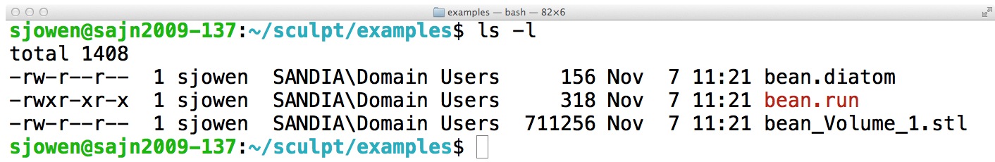
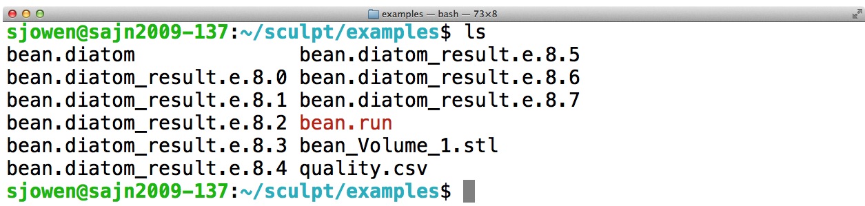
cd "path/to/my/sculpt/examples" |
delete mesh |
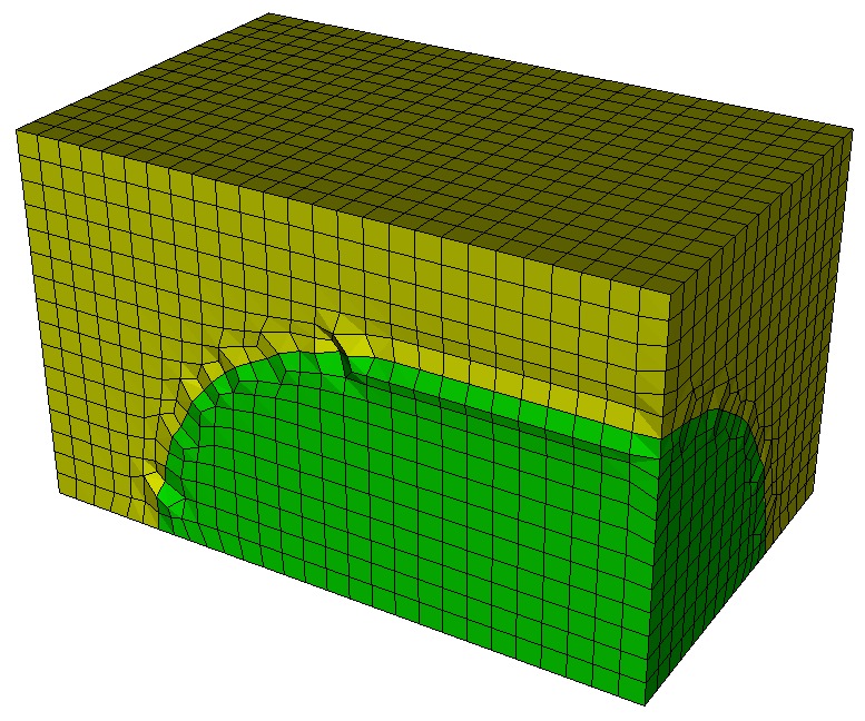
In this case, we used the no_execute option which does not invoke the Sculpt application. Instead it will write a series of files to the working directory. The fileroot option defines the base file name for the files that will be written; in this case "bean". We also use the processors option to set the number of processors to be used to 8.
bean.diatom: Diatoms is a file format used by Sandia’s CTH and Alegra analysis programs that includes a rich constructive solid geometry definition. A series of directives for constructing and orienting primitives to build a complete solid model can be used. Included in the Diatom description is an STL import option. While any standard Diatom description may be used as input to Sculpt, for Cubit’s purposes, only the STL option is used. This file contains a listing of all STL files that will be used as input to Sculpt.
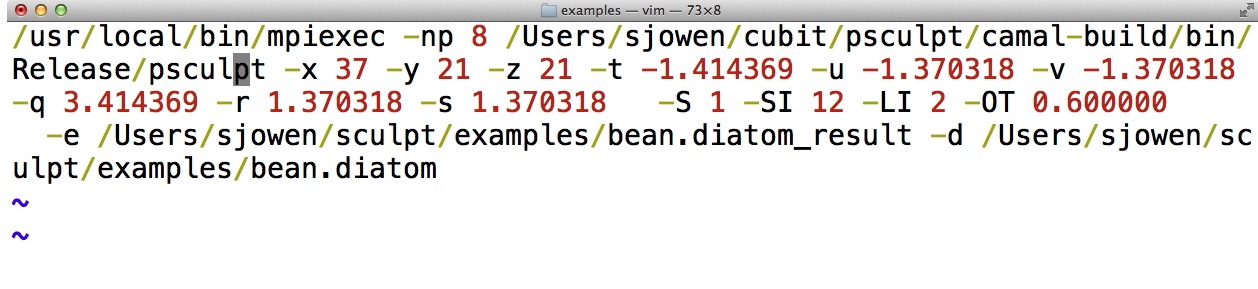
bean.run: The .run file contains the unix command line for running sculpt. Note that the file permissions have been set to execute to allow this file to be used as a unix script. Figure 248 shows the .run file for this example. Note that the command uses mpiexec and the psculpt executables, along with their full path. These paths may need to be edited when running on a different machine. It also includes the default parameters for setting the sizes, bounding box and smoothing parameters that have been computed by Cubit.
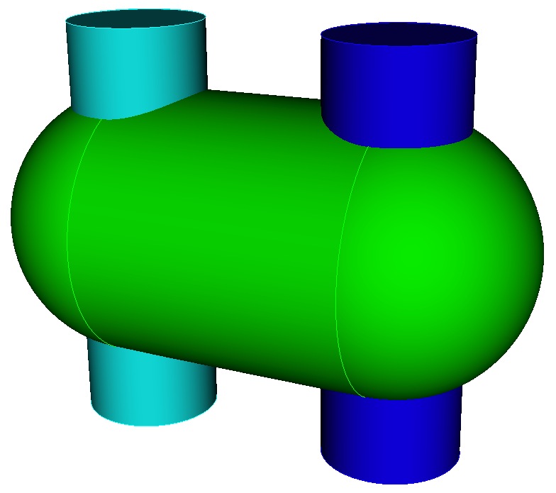
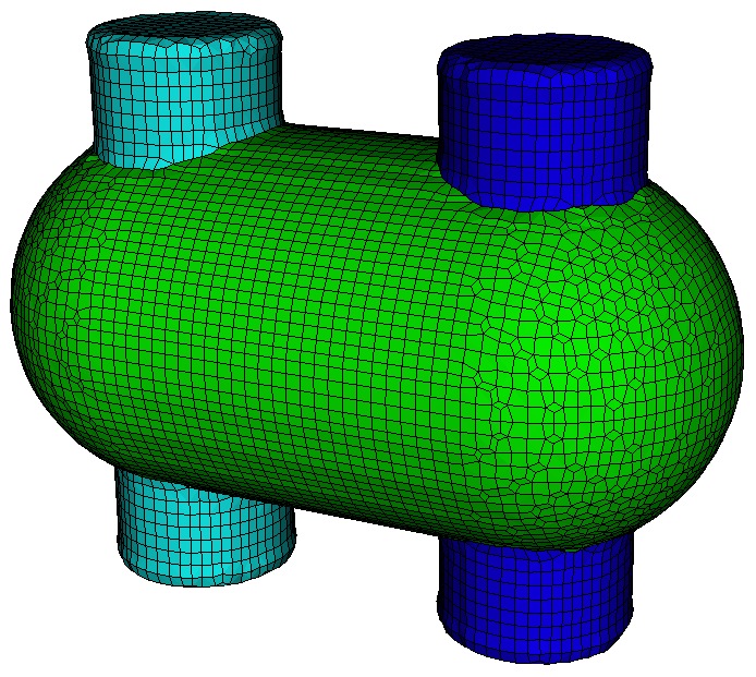
bean_Volume_1.stl: The STL file is a copy of the geometric model. In our case, it is a representation of the cylinder and sphere object we have been working with. The STL format is a set of triangles that describe the surfaces of the object. One STL file will be generated for each Volume. If the Block option is used, then one file for each Block would be created.
./bean.run |
If Sculpt is to be run on a different machine, copy the files in the working directory to the other machine and issue the same command. Remember to change the path to the mpiexec and psculpt executables to match those on the new machine. For running on cluster machines that have scheduling of resources, check with your system administrator for how to submit a job for running.
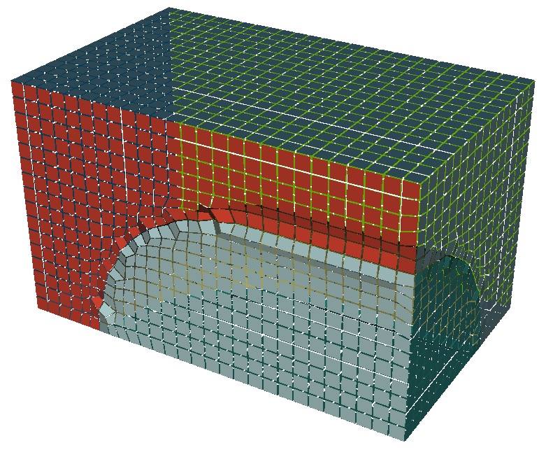
Note that 8 exodus files have been generated, 1 from each processor. These files can be used by themselves or used as-is for use in a simlation, or they can be combined into a single file. The exodus files produced by Sculpt include all appropriate parallel communication information as defined by the Nemesis format. Nemesis is an extension of Sandia’s Exodus II format that also includes appropriate parallel communication information.
epu -p 8 bean.diatom_result |
import mesh "bean.diatom_result.e" no_geom |
The result should be the same mesh we generated previously that is shown in Figure 243.
5.4.11.1.6.6 Meshing Multiple Materials With Sculpt
delete mesh |
sculpt parallel size 0.075 |
We should also note that imprint/merge operations typically needed, were also not required. While it is usually best to avoid overlaps to avoid ambiguities in the topology, Sculpt is able to generate a mesh giving precedence to the most recently defined materials. Merging is performed strictly by geometric proximity. Volumes closer than about one half the user input size will normally be automatically merged.
quality hex all scaled jacobian draw mesh |
delete mesh |
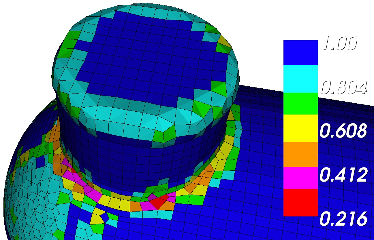
Figure 255: Cutaway of mesh reveals the additional layer of hexes surrounding each surface when the pillow option is used.
5.4.11.2 Sculpt Adaptive Meshing
Sculpt options for specifying adaptive meshing. Sculpt uses an initial overlay Cartesian grid that serves as the basis for the all-hex mesh. The default mesh size will roughly follow the constant size cells of the overlay grid. The adaptivity option allows the user to automatically split cells of the Cartesian grid based on geometric criteria, resulting in smaller cells in regions with finer details. The adapted grid is then used as the basis for the Sculpt procedure.
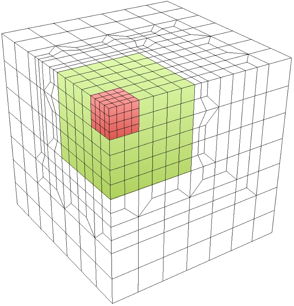
Adaptive mesh begins with constant size coarse Cartesian grid. Cells are recursively split based on geometry criteria and transitions added between levels. Projections and smoothing are performed to improve element quality.
Three options are used for controlling the adaptivity in sculpt: adapt_type, adapt_levels and adapt_threshold. The adapt_type option controls the method and geometric criteria used for deciding which cells to split in the grid, while the adapt_levels option controls the the maximum number of times any one cell can be split. Depending upon the adapt_type selected, the adapt_threshold is used as the specific geometric threshold value at which the decision is made to split any given cell.
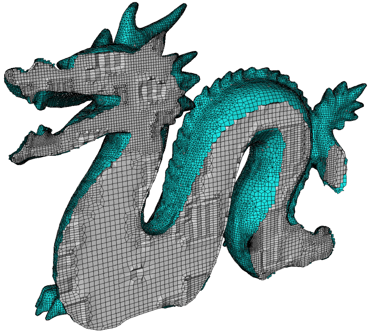
Figure 257: Initial cut-away view of adapted grid from dragon model before performing Sculpt operations.
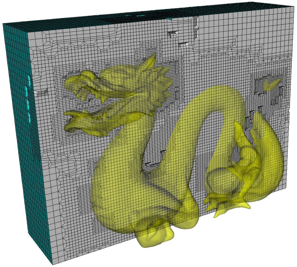
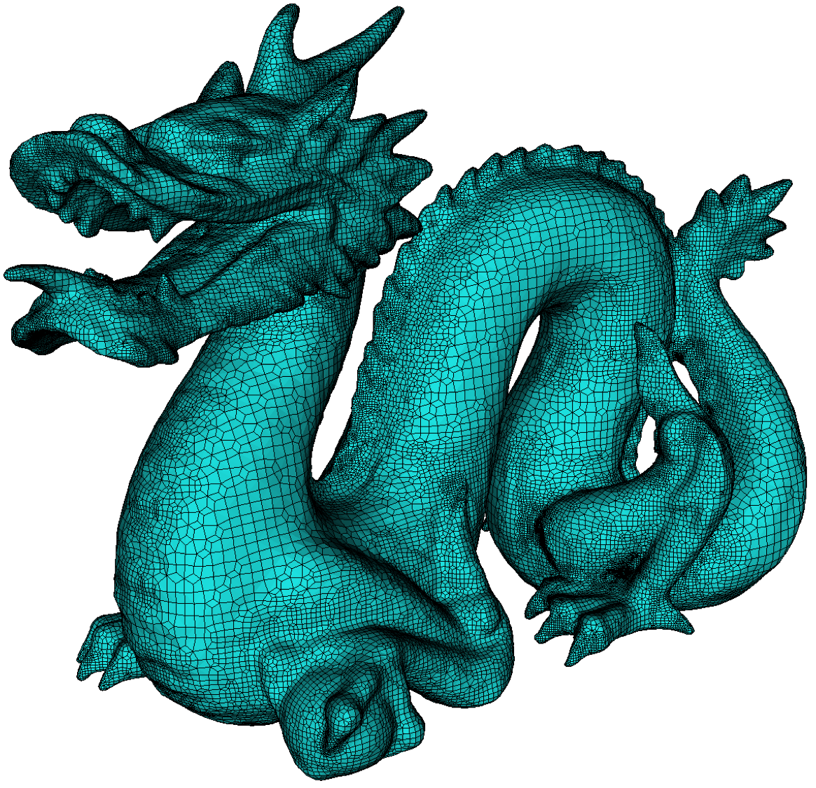
Figure 258: The final mesh of the dragon model and cutaway view of the mesh is shown with up to 4 levels of adaptive refinement.
Adaptive Meshing --adapt -adp |
--adapt_type -A <arg> Adaptive meshing type |
--adapt_threshold -AT <arg> Threshold for adaptive meshing |
--adapt_levels -AL <arg> Number of levels of adaptive refinement |
--adapt_export -AE Export exodus mesh of refined grid |
--adapt_non_manifold -ANM Refine at non-manifold conditions |
5.4.11.2.1 Adaptive Refinement Type
ommand: adapt_type Adaptive meshing type |
Input file command: adapt_type <arg> |
Command line options: -A <arg> |
Argument Type: integer (0, 1, 2, 3, 4, 5) |
Input arguments: off (0) |
facet_to_surface (1) |
surface_to_facet (2) |
surface_to_surface (3) |
vfrac_average (4) |
coarsen (5) |
vfrac_diff (6) |
vfrac_difference (6) |
Command Description:
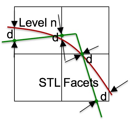
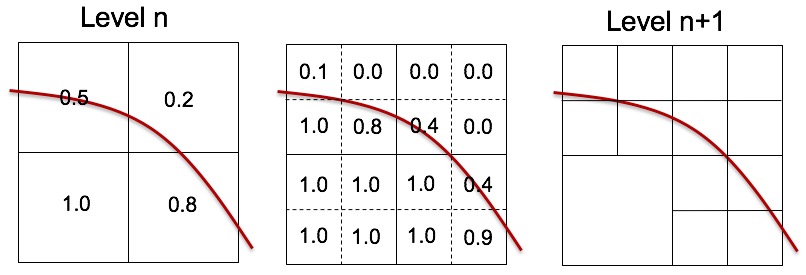
This option will automatically refine the mesh according to a user-defined criteria. Without this option, a constant cell size will be assumed everywhere in the model. To build the mesh, Sculpt uses an approximation to the exact geometry of the CAD model by interpolating mesh surfaces from volume fraction samples in each cell of the Cartesian grid. In general, the, higher the resolution of the Cartesian grid, the more sampling is done and the more accurate the mesh will represent the initial geometry. The adapt_type selected will control the criteria used for refining the mesh. If the criteria is not satisfied, the refinement will continue until a threshold indicated by the adapt_threshold parameter is satisfied everywhere, or the maximum number of levels (adapt_levels) is reached. The following criteria for refinement are available:
off (0): Cartesian grid is defined only by nelx, nely, and nelz or cell_size which is used as the basis for the sculpt mesh. No refinement will be performed.
facet_to_surface (1): This option will evaluate every location where an edge in the Cartesian grid intersects a triangle of the STL model and measures the closest distance to the approximated geometry. The cells adjacent to intersecting edges where the measured distance is greater than the adapt_threshold will be identified for uniform refinement. This is done for each refinement level where a new approximated geometry is then computed based upon the finer resolution grid. The refinement will continue until all measured distances are less than the adapt_threshold, or the maximum number of levels (adapt_levels) is reached. This option can only be used if input comes from an STL file. Microstructures and diatoms are currently not supported.
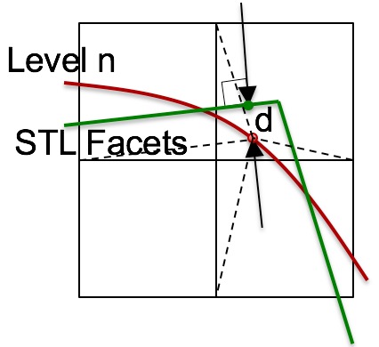
surface_to_facet (2): This criteria is similar to facet_to_surface (1) except that the locations selected for sampling are chosen from the vertices representing the approximated surfaces. The closest distance measured to any of the facets in the STL model is used as the criteria for refinement. Those cells at vertices where the distance measured exceeds the adapt_threshold are identified for refinement. This option is generally faster than 1, but may miss features if the initial resolution of the grid is too coarse. This option can also only be used if input geometry comes from an STL file. Microstructures and diatoms are currently not supported.
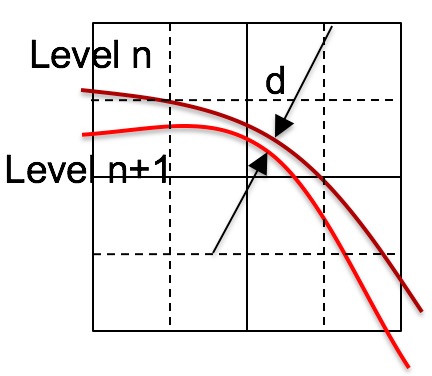
surface_to_surface (3): This criteria will test each cell to compute the local interpolated surface for the cell and compare with the surface interpolated for its eight subdivided child cells. If the distance between these two approximated surfaces is greater the the user defined adapt_threshold, then the cell will be uniformly refined. This option can be used with STL and diatom input geometry, but not with Microstructures.
vfrac_average (4): Each cell of the Cartesian grid is tested to determine if it should be subdivided into eight cells. The volume fraction of the parent cell is compared with the average volume fraction of its eight child cells. If the absolute difference between the average child volume fraction and its parent volume fraction is greater than the user defined adapt_threshold then the cell is uniformly refined. The adapt_threshold for this case should be a number between 0 and 1. A smaller number will be more sensitive to changes in geometry, usually resulting in more refinement at interfaces.
coarsen (5): Given a dense set of data on a Cartesian Grid, Sculpt will begin at a coarse resolution and refine to capture changes in the data. It uses the adapt_levels option to determine the coarseness of the initial grid. For example, a dense grid of LxMxN cells will begin with an initial resolution of L/2^a x M/2^a x N/2^a, where a is the user defined adapt_levels value. Cells will be identified for refinement if the volume fraction of any material in a cell is greater than the user defined adapt_threshold and less than 1.0-adapt_threshold. This option is available only for input_spn and input_micro formats. It is most useful for cases where very dense data is initially provided which would be too fine to serve as an FEA mesh. This method will effectively coarsen the mesh on the interior and exterior of solids, but maintain a fine resolution at geometry boundaries.
Refine to Dense Data (Coarsening). Initial grid at resolution N X M is coarsened to N0 X M0 based on the adapt_levels value. Coarse cells are then split similar to criteria in adapt_type = 4.
vfrac_difference (6): Each cell of the Cartesian grid is tested to determine if it should be subdivided into eight cells. The volume fraction of the parent cell is compared with each of the volume fractions of its eight child cells. If the absolute difference between any of the child volume fractions and its parent volume fraction is greater than the user defined adapt_threshold then the cell is uniformly refined. The adapt_threshold for this case should be a number between 0 and 1. A smaller number will be more sensitive to changes in geometry, usually resulting in more refinement at interfaces.
To maintain a conforming mesh, transition elements will be inserted to transition between smaller and larger element sizes. Default for the adapt_type option is off (0) (or that no adaptive refinement will take place).
In all cases the initial Cartesian grid defined by xint, yint and zint or the cell_size value will be used as the basis for refinement and will define the approximate largest element size in the mesh.
5.4.11.2.2 Adaptive Refinement Threshold
Command: adapt_threshold Threshold for adaptive meshing |
Input file command: adapt_threshold <arg> |
Command line options: -AT <arg> |
Argument Type: floating point value >= 0.0 |
Command Description:
This value controls the sensitivity of of the adaptivity. The value used should be based upon the adapt_type:
adapt_threshold = 0.25 * cell_size / adapt_levels^2 |
The adapt_threshold value in this case represents the maximum difference in volume fraction between a parent cell and the average of its eight child cells. This value should be between 0.0 and 1.0. The smaller the number, the more sensitive will be the adaptation and the greater the number of resulting elements. A default adapt_threshold of 0.01 is used if not specified.
facet_to_surface (1)
surface_to_facet (2)
surface_to_surface (3)
vfrac_average (4)
coarsen (5)
Note that the user defined adapt_threshold may not be satisfied everywhere in the mesh if the value defined for adapt_levels is exceeded.
5.4.11.2.3 Number of Adaptive Levels
Command: adapt_levels Number of levels of adaptive refinement |
Input file command: adapt_levels <arg> |
Command line options: -AL <arg> |
Argument Type: integer >= 0 |
Command Description:
number of cells = 8^adapt_levels |
min cell edge length = cell_size / adapt_levels^2 |
The actual number of refinement levels used will be determined by whether all cells meet the adapt_threshold, or the adapt_levels value is exceeded. The default adapt_levels is 2. Note that setting the adapt_levels more than 4 or 5 can result in long compute times.
5.4.11.2.4 Export Refined Cartesian Grid
Command: adapt_export Export exodus mesh of refined grid |
Input file command: adapt_export |
Command line options: -AE |
Command Description:
Export an exodus mesh containing the refined Cartesian grid. Interface reconstruction, boundary layer insertion and smoothing have not yet been applied to this mesh. It is the base mesh used as input to Sculpt. One file per processor will be exported in the form "vfrac_adapt.e.x.x". The exodus mesh produced will also contain the computed volume fractions for each material present in the model represented as element variables.
This option is primarily used for debugging the refinement option. However the mesh produced with this option can be used as the base mesh when used with the input_mesh option. For example, instead of Cartesian grid options, the input mesh may be specified as input_mesh = vfrac_adapt.e.1.0. Sculpt will use the refined mesh and the volume fraction element variables to build the final mesh.
5.4.11.2.5 Adapt Cells at Non-manifold Nodes
Command: adapt_non_manifold Refine at non-manifold conditions |
Input file command: adapt_non_manifold |
Command line options: -ANM |
Command Description:
If refinement results in a non-manifold condition at a node, the surrounding cells will be identified for refinement. In some cases, using this option will result in a closer match to geometry for thin layers or small features. Using this option will normally result in more elements at material interfaces. Note that in all cases non-manifold conditions will be resolved even without this option in a subsequent step, however without this option, the resulting solution may not match geometry as accurately.
The adapt_non_manifold option is off by default. It is currently only implemented for adapt_type that use an STL geometry definition. (adapt_type = 1,2,3)
5.4.11.3 Sculpt Application
This page describes the Sculpt application, a separate companion application to Cubit designed to run in parallel for generating all-hex meshes of complex geometry. Sculpt was developed as a separate application so that it can be run independently from Cubit on high performance computing platforms. It was also designed as a separable software library so it can be easily integrated as an in-situ meshing solution within other codes. As installed with Cubit, Sculpt can be set up and run directly from Cubit, in a batch process from the unix command line or from a user-defined input file. This documentation describes the input file and command line syntax for the Sculpt Application when running in batch mode. See this page for using Cubit to set up input for Sculpt. A brief technical description of Sculpt may also be found here.
5.4.11.3.1 Sculpt System Requirements
Sculpt is currently built for windows, linux and mac operating systems. Current supported OS versions should be the same as those supported by Cubit. It is designed to take advantage of 64 bit multicore and distributed memory computers, using open-mpi as the basis for parallel communications.
5.4.11.3.2 Running Sculpt
Sculpt can be run using one of two excutables:
psculpt requires the use of mpiexec to start the process. Number of processors to use is specified by the -np argument to mpiexec. psculpt and its input parameters are also used as input to mpiexec. For example:
mpiexec -np 8 psculpt -stl myfile.stl -cs 0.5 |
If appropriate system paths have not been set, you may need to use full paths when referring to mpiexec and psculpt.
This application assumes that mpiexec is included in the standard CUBIT installation directory. The number of processors to use is specified by the -j option. For example: sculpt -j 8 -stl myfile.stl -cs 0.5 If the -j option is not used, sculpt will default to a single processor for execution. The -mpi option can also be used with the sculpt application to indicate a specific mpi installation that is not included with CUBIT. For example:
sculpt -j 8 -mpi /path/to/mpiexec -stl myfile.stl -cs 0.5 |
5.4.11.3.3 Sculpt Examples
The following illustrate simple use cases of the Sculpt application. To use these examples, copy the following stl and diatom files to your working directory:
brick1.stl
brick2.stl
bricks.diatom
5.4.11.3.3.1 Example 1
sculpt -j 4 -stl brick1.stl -cs 0.5
brick1.stl_results.e.4.0 |
brick1.stl_results.e.4.1 |
brick1.stl_results.e.4.2 |
nbrick1.stl_results.e.4.3 |
epu -p 4 brick1.stl_results |
brick1.stl_results.e |
To view the resulting mesh in Cubit, use the import free mesh command. For example:
import mesh "brick1.stl_results.e" no_geom |
5.4.11.3.3.2 Example 2
mpiexec -np 4 psculpt -x 46 -y 26 -z 26 -t -6.5 -u -6.5 -v -6.5 -q 16.5 -r 6.5 -s 6.50 -d bricks.diatom |
In this case we use mpiexec to start 4 processes of psculpt. We explicitly define the number of Cartesian intervals and the dimensions of the grid. Rather than using the -stl option, we use the -d option which allows us to specify the diatom file, bricks.diatom. This file allows us to specify multiple stl files, where each one represents a different material. In this case we use both brick1.stl and brick2.stl, which are called out in bricks.diatom.
5.4.11.4 Sculpt Boundary Conditions
Sculpt options for specifying the methods for generating nodesets, sidesets and blocks on the mesh. Several automatic methods for generating nodesets and sidesets are provided in Sculpt using the gen_sidesets option. Where multiple blocks are required, Block IDs are normally defined using the material ID in the diatom file. Each STL file can be associated with a different block ID. If the mesh_void option is used, the ID for the block of elements in the void region can be set using the void_mat option.
oundary Conditions --boundary_condition -bc |
--void_mat -VM <arg> Void material ID (when mesh_void=true) |
--separate_void_blocks -SVB Separate void into unique block IDs |
--gen_sidesets -SS <arg> Generate sidesets |
--free_surface_sideset -FS <arg> Free Surface Sideset |
--match_sidesets -mss <arg> Sidesets ids of matching pairs |
5.4.11.4.1 Void Material ID
Command: void_mat Void material ID (when mesh_void=true) |
|
Input file command: void_mat <arg> |
Command line options: -VM <arg> |
Argument Type: integer > 0 |
Command Description:
When the mesh_void option is used, this value is the material (block) ID assigned to all elements in the void region. If void_mat option is not used, the material ID of elements in the void region will be the maximum material ID in the model + 1. Note that the void_mat may be the same as an existing material in another part of the model.
5.4.11.4.2 Separate Void Blocks
ommand: separate_void_blocks Separate void into unique block IDs |
|
Input file command: separate_void_blocks |
Command line options: -SVB |
Command Description:
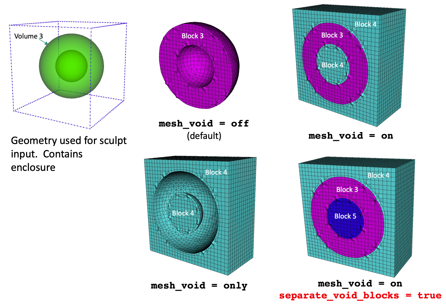
5.4.11.4.3 Generate Sidesets
Command: gen_sidesets Generate sidesets |
|
Input file command: gen_sidesets <arg> |
Command line options: -SS <arg> |
Argument Type: integer (0, 1, 2, 3, 4, 5) |
Input arguments: off (0) |
fixed (1) |
variable (2) |
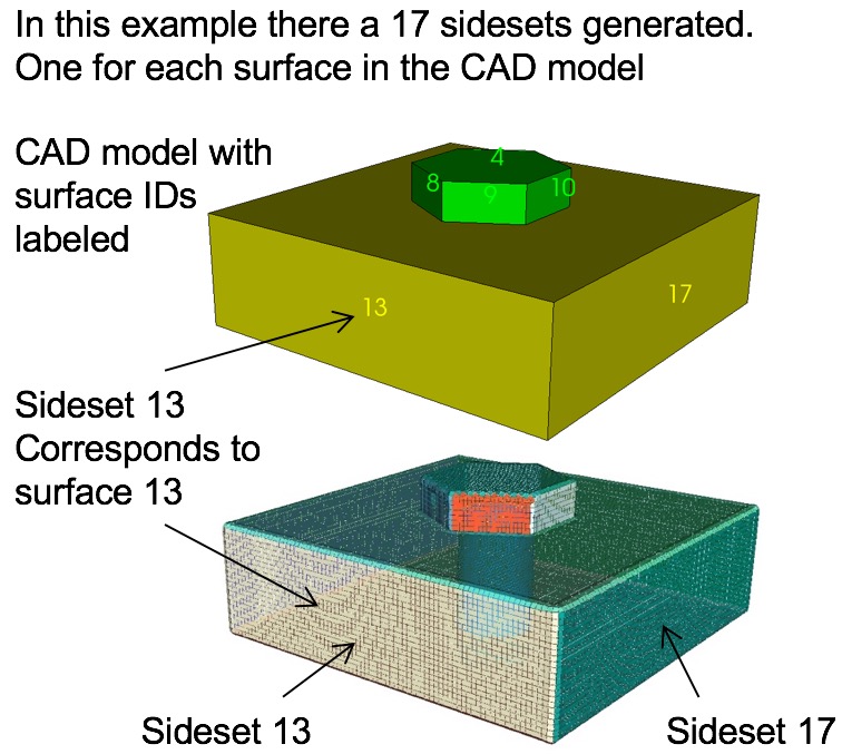
geometric_surfaces (3) |
geometric_sidesets (4) |
rve (5) |
input_mesh_and_stl (6) |
input_mesh_and_free_surfaces (7) |
rve_variable (8) |
Generate exodus sidesets using one of the following options:
off (0): No sidesets will be generated
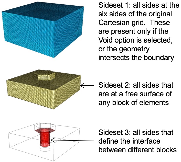
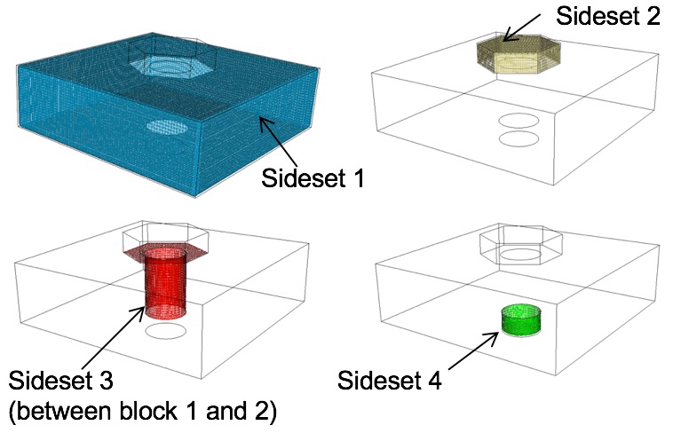
fixed (1): Exactly 3 sidesets will be generated according to the following:
Sideset 1: All sides at the domain boundary. Sides will only be present in this sideset if the model intersects the enclosing bounding box or the void option is used.
Sideset 2: All sides at the model boundary. Any side on the model that is not interior will be included. This should represent a full enclosure of the model if it does not intersect the domain boundary.
Sideset 3: All sides at material interfaces. Includes sides on the interior where adjacent blocks are different.
variable (2): A variable number of sidesets will be generated with the following characteristics:
Surfaces at the domain boundary
Exterior material surfaces
Interfaces between materials
surface |
1 0 1 2 3 4 5 6 7 8 9 |
10 11 12 13 14 15 16 17 18 19 |
20 21 22 23 |
endsurface 1 |
Nodeset/Sideset ID Contains nodes/faces |
1 on minimum X domain boundary |
2 on maximum X domain boundary |
3 on minimum Y domain boundary |
4 on maximum Y domain boundary |
5 on minimum Z domain boundary |
6 on maximum Z domain boundary |
In addition, a nodeset and sideset will be generated on interior surfaces for each unique pair of adjacent material IDs. One final nodeset will also be generated along interior curves at all internal triple junctions (curves where at least 3 surfaces share a common curve).
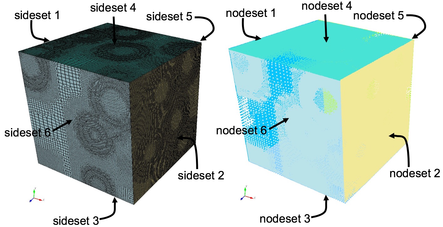
Figure 272: Example of automatically defined sidesets at domain boundaries of an RVE and at all interface surfaces between materials.
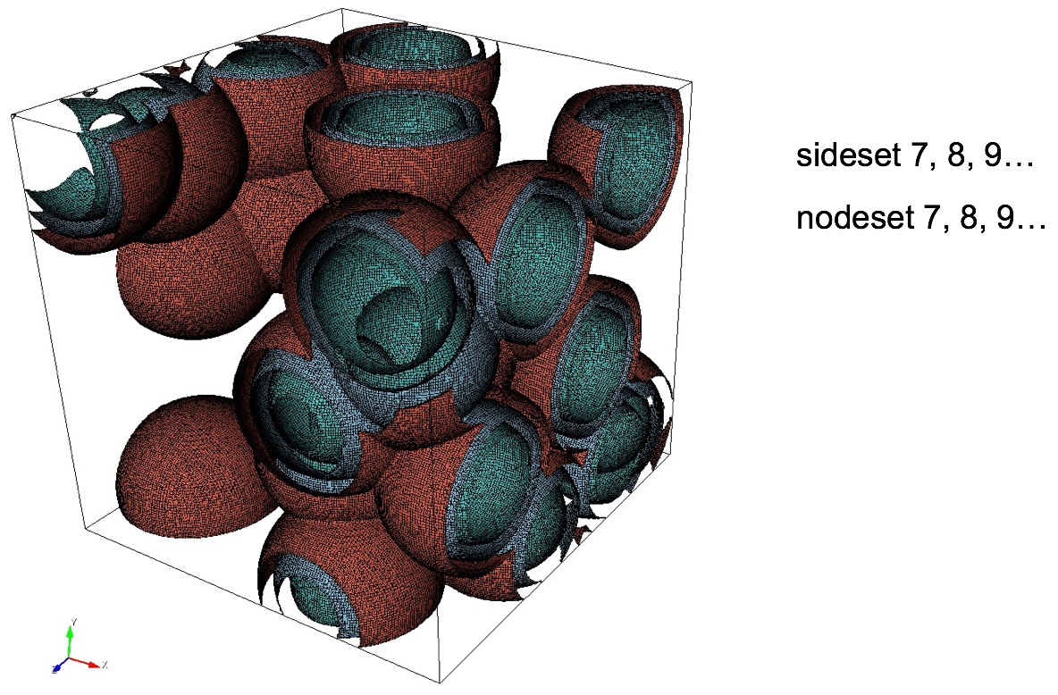
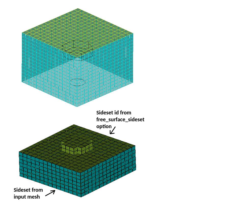
Figure 273: Example of sidesets defined in the input mesh and corresponding domain boundary sidesets in the output mesh.
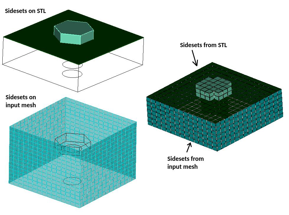
Figure 274: Example of sidesets defined in the input mesh and corresponding domain boundary sidesets in the output mesh.
rve_variable (8): Nodesets 1-6 and Sidesets 1-6 are defined at the boundaries as described in the gen_sidesets = rve (5) option. With the rve_variable option, additional nodesets and sidesets at material interfaces on the interior of the mesh are defined similar to the gen_sidesets = variable (2) option. Grouping of interior sides in a sidesets will be contiguous, where a separate sideset will be generated for each unique set of contiguous sides. Nodesets will be generated in a similar manner.
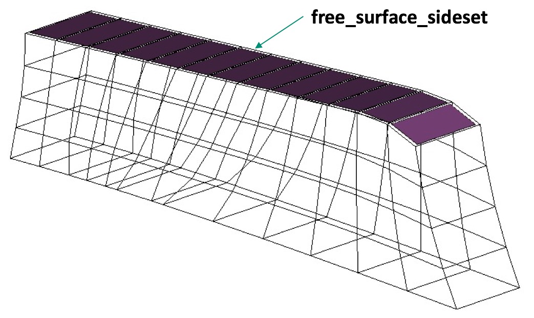
5.4.11.4.4 Free Surface Sidesets
Command: free_surface_sideset Free Surface Sideset |
|
Input file command: free_surface_sideset <arg> |
Command line options: -FS <arg> |
Argument Type: integer(s) >= 0 |
Command Description:
Given exodus sidesets are treated as interior surfaces for STL projection.
5.4.11.4.5 Match Sideset Ids
Command: match_sidesets Sidesets ids of matching pairs |
|
Input file command: match_sidesets <arg> |
Command line options: -mss <arg> |
Argument Type: integer(s) >= 0 |
Command Description:
If used with an unstructured base grid (input mesh), this option allows the user to define a crack in the input mesh, where the faces of each vertical side (wall) of the crack are each in a different sideset. The faces at the bottom of the crack share a common edge (V-bottom) or face (square-bottom). Sculpt will match or equalize the volume fractions of the bottom cells on either side of the crack. This produces a uniform, higher quality mesh at the crack. The sidesets must be specified in a pairwise order. This option must be used with the –input_mesh (-im) option.
5.4.11.5 Sculpt Boundary Layers
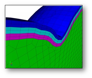
Figure 277: Boundary layers defined at the surfaces of a material.
Boundary Layers --boundary_layer -bly |
--begin -beg <arg> Begin specification blayer or blayer_block |
--end -zzz <arg> End specification blayer or blayer_block |
--material -mat <arg> Boundary layer material specification |
--num_elem_layers -nel <arg> Number of element layers in blayer block |
--thickness -th <arg> Thickness of first element layer in block |
--bias -bi <arg> Bias of element thicknesses in blayer block |
5.4.11.5.1 Boundary Layer Begin
Command: begin Begin specification blayer or blayer_block |
Input file command: begin <arg> |
Command line options: -beg <arg> |
Argument Type: blayer, blayer_block |
Command Description:
Defines the beginning of a specification block. Must be closed with "end" argument. Currently supports the following specifications:
blayer
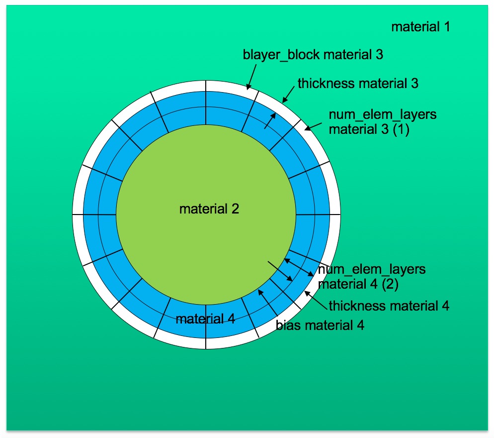
Defines a boundary layer specification. Layers of hex elements are placed at the interface of a given material. Valid argumnts used within a blayer specification include: material, and begin blayer_block.
blayer_block
Defines a set of element layers within a given blayer definition that share a common material ID. Valid arguments used within a blayer_block specification include: material, num_elem_layers, thickness and bias.
The following example shows a boundary layer specification in a sculpt input file. In this example, two boundary layer blocks are defined at the interface of materials 1 and 2. Two material blocks with ID 3 and 4 are generated with 1 and 2 element layers respectively.
BEGIN BLAYER |
MATERIAL = 1 2 |
BEGIN BLAYER_BLOCK |
MATERIAL = 3 |
NUM_ELEM_LAYERS = 1 |
THICKNESS = 0.1 |
END BLAYER_BLOCK |
BEGIN BLAYER_BLOCK |
MATERIAL = 4 |
NUM_ELEM_LAYERS = 2 |
THICKNESS = 0.2 |
BIAS = 1.3 |
END BLAYER_BLOCK |
END BLAYER |
5.4.11.5.2 Boundary Layer End
Command: end End specification blayer or blayer_block |
Input file command: end <arg> |
Command line options: -zzz <arg> |
Argument Type: blayer, blayer_block |
Command Description:
Defines the end of a specification block. Must be preceded with "begin" argument. Currently supports arguments blayer and blayer_block.
5.4.11.5.3 Boundary Layer Material
Command: material Boundary layer material specification |
Input file command: material <arg> |
Command line options: -mat <arg> |
Argument Type: integer > 0 |
Command Description:
Defines a material ID in a boundary layer specification. When used within a BLAYER specification, it references one or two existing materials in the input where boundary layers will be generated. If a single material is specified, hex layers will be generated at all interfaces of the designated material with any adjacent material. If two material IDs are specified, layers will be generated only at interfaces where the two materials are adjacent.
In most cases, the material ID(s) in the BLAYER specification refer to material IDs defined in the diatom file for specific geometry inserts such as STL files or diatom primitives. It can also be defined as the void material ID (VOID_MAT) or a material in a volume fraction description such as input_vfrac, input_micro, input_cart_exo or input_spn.
When used within a BLAYER_BLOCK specification, it refers to a new block that will be generated for which all elements in the blayer_block will be assigned. Normally it refers to a unique material ID that is not already referenced in the input. Where the material ID is already used, elements in the blayer block will be added to the existing material.
A material ID must be defined for both a BLAYER and BLAYER_BLOCK. This value does not have a default.
5.4.11.5.4 Number of Element Layers in Boundary Layer
Command: num_elem_layers Number of element layers in blayer block |
Input file command: num_elem_layers <arg> |
Command line options: -nel <arg> |
Argument Type: integer > 0 |
Command Description:
Number of element layers to be defined within a BLAYER_BLOCK specification. num_elem_layers must be defined for all BLAYER_BLOCKs.
5.4.11.5.5 Boundary Layer Thickness
ommand: thickness Thickness of first element layer in block |
Input file command: thickness <arg> |
Command line options: -th <arg> |
Argument Type: floating point value |
Command Description:
Thickness of the first layer defined in a BLAYER_BLOCK. Value is an absolute distance. No default is provided and must be defined for all BLAYER_BLOCKs
5.4.11.5.6 Boundary Layer Bias
Command: bias Bias of element thicknesses in blayer block |
Input file command: bias <arg> |
Command line options: -bi <arg> |
Argument Type: floating point value |
Command Description:
Bias factor applied to additional layers of a BLAYER_BLOCK. Used in conjunction with the THICKNESS parameter (thickness of first layer) it defines a multiplier for the thickness for subsequent element layers defined within the same BLAYER_BLOCK. Default BIAS is 1.0 and is optional.
5.4.11.6 Sculpt Command Summary
Following is a listing of the available input commands to either sculpt or psculpt. When used from the unix command line, commands may be issued using the short form argument, designated with a single dash(-), or with the longer form, designated with two dashes (–). When used in an input file, only the long form may be used, omitting the two dashes (–)
Process Control --process -pc |
--num_procs -j <arg> Number of processors requested |
--input_file -i <arg> File containing user input data |
--debug_processor -D <arg> Sleep to attach to processor for debug |
--debug_flag -dbf <arg> Dump debug info based on flag |
--quiet -qt Suppress output |
--print_input -pi Print input values and defaults then stop |
--version -vs Print version number and exit |
--threads_process -tpp <arg> Number of threads per process |
--iproc -ip <arg> Number of processors in I direction |
--jproc -jp <arg> Number of processors in J direction |
--kproc -kp <arg> Number of processors in K direction |
--periodic -per Generate periodic mesh |
--check_periodic -cp <arg> Check for periodic geometry |
--check_periodic_tol -cpt <arg> Tolerance for checking periodicity |
--periodic_axis -pax <arg> Axis periodicity is about |
--periodic_nodesets -pns <arg> Nodesets ids of master/slave nodesets |
--build_ghosts -bg Write ghost layers to exodus files for debug |
--vfrac_method -vm <arg> Set method for computing volume fractions |
|
Input Data Files --input -inp |
--stl_file -stl <arg> Input STL file |
--diatom_file -d <arg> Input Diatom description file |
--input_vfrac -ivf <arg> Input from Volume Fraction file base name |
--input_micro -ims <arg> Input from Microstructure file |
--input_cart_exo -ice <arg> Input from Cartesian Exodus file |
--input_spn -isp <arg> Input from Microstructure spn file |
--spn_xyz_order -spo <arg> Ordering of cells in spn file |
--lattice -l <arg> STL Lattice Template File |
|
Output --output -out |
--exodus_file -e <arg> Output Exodus file base name |
--volfrac_file -vf <arg> Output Volume Fraction file base name |
--quality -Q Dump quality metrics to file |
--export_comm_maps -C Export parallel comm maps to debug exo files |
--write_geom -G Write geometry associativity file |
--write_mbg -M Write mesh based geometry file <beta> |
--compare_volume -cv Report vfrac and mesh volume comparison |
--compute_ss_stats -css Report sideset statistics |
|
Overlay Grid Specification --overlay -ovr |
--nelx -x <arg> Num cells in X in overlay Cartesian grid |
--nely -y <arg> Num cells in Y in overlay Cartesian grid |
--nelz -z <arg> Num cells in Z in overlay Cartesian grid |
--xmin -t <arg> Min X coord of overlay Cartesian grid |
--ymin -u <arg> Min Y coord of overlay Cartesian grid |
--zmin -v <arg> Min Z coord of overlay Cartesian grid |
--xmax -q <arg> Max X coord of overlay Cartesian grid |
--ymax -r <arg> Max Y coord of overlay Cartesian grid |
--zmax -s <arg> Max Z coord of overlay Cartesian grid |
--cell_size -cs <arg> Cell size (nelx, nely, nelz ignored) |
--align -a Automatically align geometry to grid |
--bbox_expand -be <arg> Expand tight bbox by percent |
--input_mesh -im <arg> Input Base Exodus mesh |
--input_mesh_blocks -imb <arg> Block ids of Input Base Exodus mesh |
--input_mesh_material -imm <arg> Material definition with input mesh |
--input_mesh_pamgen -imp <arg> Input Base mesh defined by Pamgen |
|
Mesh Type --type -typ |
--stair -str <arg> Generate Stair-step mesh |
--mesh_void -V <arg> Mesh void |
--trimesh -tri Generate tri mesh of geometry surfaces |
--tetmesh -tet <arg> Under Development |
--deg_threshold -dg <arg> Convert hexes below threshold to degenerates |
--max_deg_iters -dgi <arg> Maximum number of degenerate iterations |
--htet -ht <arg> Convert hexes below quality threshold to tets |
--htet_method -hti <arg> Method used for splitting hexes to tets |
--htet_material -htm <arg> Convert hexes in given materials to tets |
--htet_transition -htt <arg> Transition method between hexes and tets |
--htet_pyramid -htp <arg> Local transition pyramid |
--htet_tied_contact -htc <arg> Local transition tied contact |
--htet_no_interface -htn <arg> Local transition none |
|
Boundary Conditions --boundary_condition -bc |
--void_mat -VM <arg> Void material ID (when mesh_void=true) |
--separate_void_blocks -SVB Separate void into unique block IDs |
--gen_sidesets -SS <arg> Generate sidesets |
--free_surface_sideset -FS <arg> Free Surface Sideset |
--match_sidesets -mss <arg> Sidesets ids of matching pairs |
|
Adaptive Meshing --adapt -adp |
--adapt_type -A <arg> Adaptive meshing type |
--adapt_threshold -AT <arg> Threshold for adaptive meshing |
--adapt_levels -AL <arg> Number of levels of adaptive refinement |
--adapt_export -AE Export exodus mesh of refined grid |
--adapt_non_manifold -ANM Refine at non-manifold conditions |
|
Smoothing --smoothing -smo |
--smooth -S <arg> Smoothing method |
--csmooth -CS <arg> Curve smoothing method |
--laplacian_iters -LI <arg> Number of Laplacian smoothing iterations |
--max_opt_iters -OI <arg> Max. number of parallel Jacobi opt. iters. |
--opt_threshold -OT <arg> Stopping criteria for Jacobi opt. smoothing |
--curve_opt_thresh -COT <arg> Min metric at which curves won't be honored |
--max_pcol_iters -CI <arg> Max. number of parallel coloring smooth iters. |
--pcol_threshold -CT <arg> Stopping criteria for parallel color smooth |
--max_gq_iters -GQI <arg> Max. number of guaranteed quality smooth iters. |
--gq_threshold -GQT <arg> Guaranteed quality minimum SJ threshold |
--geo_smooth_max_deviation -GSM <arg> Geo Smoothing Maximum Deviation |
|
Mesh Improvement --improve -imp |
--pillow -p <arg> Set pillow criteria (1=surfaces) |
--pillow_surfaces -ps Turn on pillowing for all surfaces |
--pillow_curves -pc Turn on pillowing for bad quality at curves |
--pillow_boundaries -pb Turn on pillowing at domain boundaries |
--pillow_curve_layers -pcl <arg> Number of elements to buffer at curves |
--pillow_curve_thresh -pct <arg> S.J. threshold to pillow hexes at curves |
--pillow_smooth_off -pso Turn off smoothing following pillow operations |
--capture -c <arg> Project to facet geometry <beta> |
--capture_angle -ca <arg> Angle at which to split surfaces <beta> |
--capture_side -sc <arg> Project to facet geometry with surface ID |
--defeature -df <arg> Apply automatic defeaturing |
--min_vol_cells -mvs <arg> Minimum number of cells in a volume |
--defeature_bbox -dbb Defeature Filtering at Bounding Box |
--defeature_iters -dfi <arg> Maximum Number of Defeaturing Iterations |
--thicken_material -thm <arg> Expand a given material into surrounding cells |
--thicken_void -thv <arg> Insert void material to remove overlap |
--micro_expand -me <arg> Expand Microstructure grid by N layers |
--micro_shave -ms Remove isolated cells at micro. boundaries |
--remove_bad -rb <arg> Remove hexes with Scaled Jacobian < threshold |
|
Mesh Transformation --transform -tfm |
--xtranslate -xtr <arg> Translate final mesh coordinates in X |
--ytranslate -ytr <arg> Translate final mesh coordinates in Y |
--ztranslate -ztr <arg> Translate final mesh coordinates in Z |
--scale -scl <arg> Scale final mesh coordinates by constant |
|
Boundary Layers --boundary_layer -bly |
--begin -beg <arg> Begin specification blayer or blayer_block |
--end -zzz <arg> End specification blayer or blayer_block |
--material -mat <arg> Boundary layer material specification |
--num_elem_layers -nel <arg> Number of element layers in blayer block |
--thickness -th <arg> Thickness of first element layer in block |
--bias -bi <arg> Bias of element thicknesses in blayer block |
5.4.11.7 Sculpt GUI
Sculpt can be run from a terminal or a GUI. Sculpt parameters are divided into 4 areas.
5.4.11.7.1 Size Parameters
|
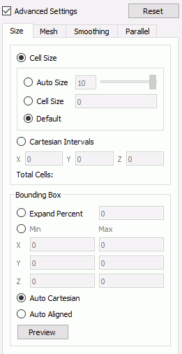
5.4.11.7.2 Mesh Parameters
|
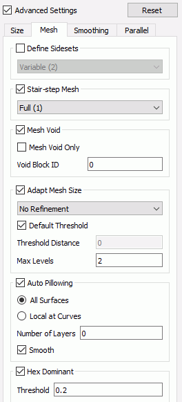
5.4.11.7.3 Smoothing Parameters
|
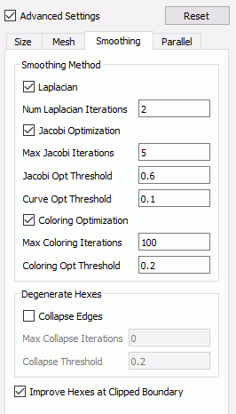
5.4.11.7.4 Parallel Parameters
|
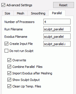
5.4.11.8 Sculpt Mesh Improvement
Sculpt options for modifying the mesh to improve mesh quality.
Mesh Improvement --improve -imp |
--pillow -p <arg> Set pillow criteria (1=surfaces) |
--pillow_surfaces -ps Turn on pillowing for all surfaces |
--pillow_curves -pc Turn on pillowing for bad quality at curves |
--pillow_boundaries -pb Turn on pillowing at domain boundaries |
--pillow_curve_layers -pcl <arg> Number of elements to buffer at curves |
--pillow_curve_thresh -pct <arg> S.J. threshold to pillow hexes at curves |
--pillow_smooth_off -pso Turn off smoothing following pillow operations |
--capture -c <arg> Project to facet geometry <beta> |
--capture_angle -ca <arg> Angle at which to split surfaces <beta> |
--capture_side -sc <arg> Project to facet geometry with surface ID |
--defeature -df <arg> Apply automatic defeaturing |
--min_vol_cells -mvs <arg> Minimum number of cells in a volume |
--defeature_bbox -dbb Defeature Filtering at Bounding Box |
--defeature_iters -dfi <arg> Maximum Number of Defeaturing Iterations |
--thicken_material -thm <arg> Expand a given material into surrounding cells |
--thicken_void -thv <arg> Insert void material to remove overlap |
--micro_expand -me <arg> Expand Microstructure grid by N layers |
--micro_shave -ms Remove isolated cells at micro. boundaries |
--remove_bad -rb <arg> Remove hexes with Scaled Jacobian < threshold |
5.4.11.8.1
#:style ’toc-hidden]{Pillow}
Command: pillow Set pillow criteria (1=surfaces) |
|
Input file command: pillow <arg> |
Command line options: -p <arg> |
Argument Type: integer (0, 1, 2, 3) |
Input arguments: off (0) |
surfaces (1) |
curves (2) |
domain_boundaries (3) |
surfaces_no_smoothing (100) |
curves_2_layers (212) |
curves_3_layers (213) |
curves_4_layers (214) |
curves_5_layers (215) |
curves_2_layers_no_smoothing (202) |
curves_3_layers_no_smoothing (203) |
curves_4_layers_no_smoothing (204) |
curves_5_layers_no_smoothing (205) |
For models that have more than one material that share an interface, unless the geometry is precisely aligned with the global axis, it is usually a good idea to turn on pillowing. Pillowing automatically inserts an additional layer of hexes at interface boundaries to improve mesh quality. Without pillowing you may notice inverted or poor quality elements at curve interfaces where 2 or more materials meet.
pillow_surfaces: Pillow around all surfaces
pillow_curves: Pillow bad quality at curves
pillow_boundaries: Pillow at domain boundaries
pillow_curve_layers: Number of element layers to buffer curves
pillow_smooth_off: Turn OFF smoothing following pillow operations
See help on the above options for more information
5.4.11.8.2 Pillow All Surfaces
sculpt-command-block{ Command: pillow_surfaces Turn on pillowing for all surfaces
Input file command: pillow_surfaces Command line options: -ps }
Command Description: Pillow option to insert a layer of hexes surrounding each internal surface in the mesh. Where two volumes share a common interface is defined as a surface. All hexes that have at least one of its faces on a surface are defined as the "shrink set" of hexes. A separate shrink set is defined for each unique surface. Hexes in the set are shrunk away from their hex neighbors not in the shrink set. A layer of hexes is then inserted surrounding all hexes in each set. This enforces the condition where no more than one hex edge will lie on any single curve thus allowing more freedom for the smoother to improve element quality.
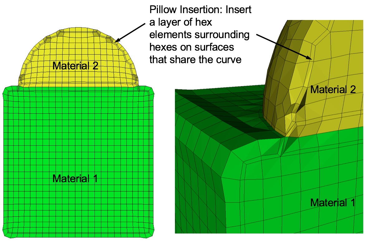
Figure 279: Example of surface pillowing, before and after smoothing
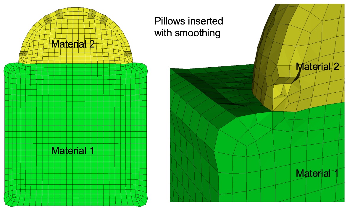
Surface pillowing is off by default. If both pillow_curves and pillow_surfaces options are used, curve pillowing will be performed before surface pillowing. See the pillow option for more information on setting additional options for pillowing.
5.4.11.8.3 Pillow Bad Quality at Curves
Command: pillow_curves Turn on pillowing for bad quality at curves |
|
Input file command: pillow_curves |
Command line options: -pc |
Command Description: Pillow option to selectively pillow hexes at curves. Only hexes that have faces with 3 or more nodes on a curve will be pillowed. Additional buffer layers of hexes beyond the poor quads at the curves will be included in the pillow region. The number of buffer layers beyond the curve can be controlled with the pillow_curve_layers, where the default will be 3 layers.
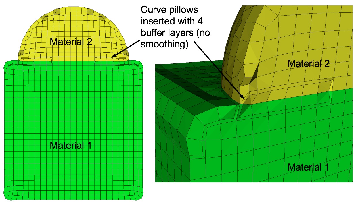
Figure 280: Example of curve pillowing with four pillow_curve_layers, before and after smoothing
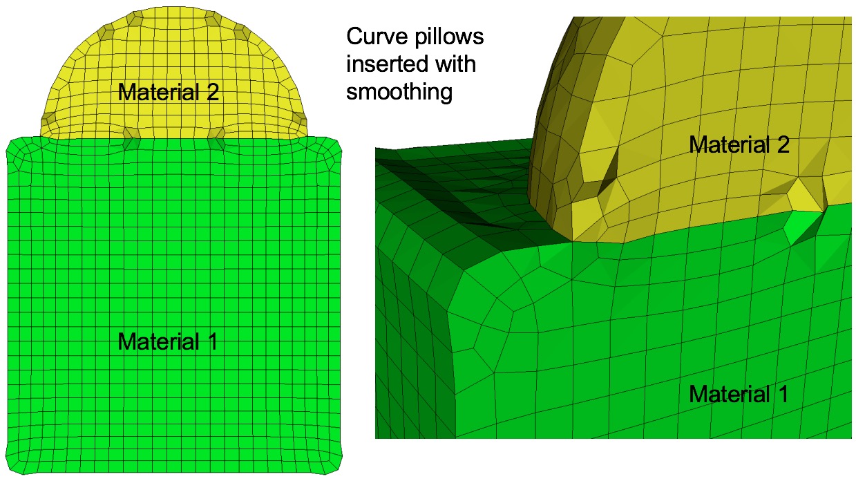
Curve pillowing is off by default. If both pillow_curves and pillow_surfaces options are used, curve pillowing will be performed before surface pillowing. See the pillow option for more information on setting additional options for pillowing.
5.4.11.8.4 Pillow at Domain Boundaries
Command: pillow_boundaries Turn on pillowing at domain boundaries |
|
Input file command: pillow_boundaries |
Command line options: -pb |
Command Description: Pillow option to insert pillow layers at domain boundaries of the initial Cartesian grid definition. One layer of hexes is inserted on each of the six faces of the Cartesian Domain. This option is useful where the void option is used to generate a mesh in the full Cartesian grid and where the adapt option has been used. Without this option, it is likely that hexes with two faces on the same domain boundary will occur if the adaptation extends to the boundary. Turning on the pillow_boundaries option should correct for these cases.
Figure 281: Example of pillowing at boundaries on a microstructure RVE. (b) before smoothing (c) after smoothing
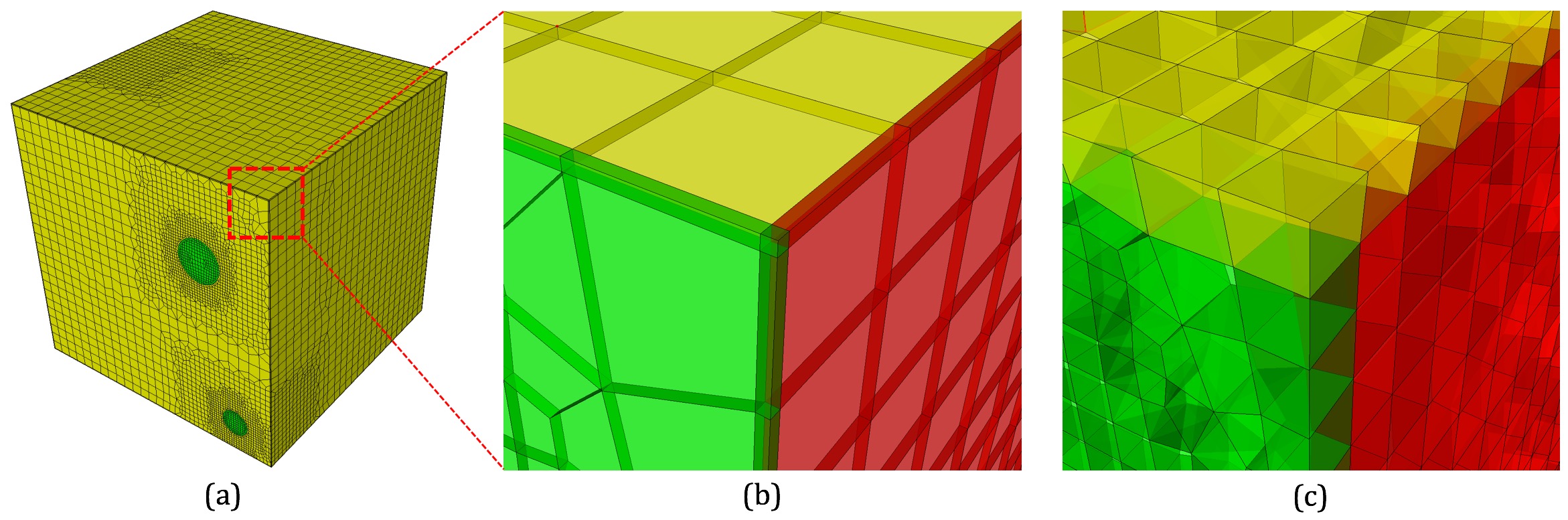
Boundary pillowing is off by default. The pillow_boundaries option may be used in the same input as pillow_surfaces or pillow_curves. The pillow_boundaries option must also be used with the mesh_void option to ensure hexes will exist at the Cartesian domain boundary. See the pillow option for more information on setting additional options for pillowing.
5.4.11.8.5 Number of Element Layers to Buffer Curves
Command: pillow_curve_layers Number of elements to buffer at curves |
|
Input file command: pillow_curve_layers <arg> |
Command line options: -pcl <arg> |
Argument Type: integer > 0 |
Command Description: Used for setting the number of buffer hex layers when the pillow_curves option is used. When pillow_curves is used a shrink set is formed from hexes that would otherwise have two or more edges on the same curve. This value will control the extent to which neighboring hexes will be included in the shrink set. The default pillow_curve_layers is 3. Setting this value lower will localize the modifications to the hex mesh, whereas, more layers will extend the region that is affected in correcting the poor quality at curves.
5.4.11.8.6 Scaled Jacobian Threshold for Curve Pillowing
Command: pillow_curve_thresh S.J. threshold to pillow hexes at curves |
|
Input file command: pillow_curve_thresh <arg> |
Command line options: -pct <arg> |
Argument Type: floating point value (-1.0->1.0) |
Command Description: Used for setting the quality threshold for pillowing hexes at curves. When determining hexes to include in the shrink set, the pillow_curves option will look for hexes with more than two nodes of a hex on the same curve. If this condition is satisfied, it will test the mesh quality of quads on the adjacent surfaces that share the common curve. If at least 3 nodes are on a common curve and the Scaled Jacobian of any of the attached quads falls below the, pillow_curve_thresh scaled Jacobian metric, then the associated hexes will be included in the shrink set.
Default for pillow_curve_thresh is 0.3. Increasing this value will tend to increase the total number of hexes added to the mesh, but may result in better mesh quality after smoothing. Lowering this value may reduce the number of additional hexes but could potentially result in more hexes with poor or bad Scaled Jacobian metrics.
5.4.11.8.7 Turn OFF Smoothing Following Pillow Operations
Command: pillow_smooth_off Turn off smoothing following pillow operations |
|
Input file command: pillow_smooth_off |
Command line options: -pso |
Command Description: Controls the smoothing following pillow operations. To maximize element quality at pillowed hexes, smoothing is always performed after inserting the hex layers. The smoothing step may be omitted if pillow_smooth_off is set. This option can be useful for visualizing the pillow layers that have been inserted, but in most cases will generate poor quality or inverted elements.
5.4.11.8.8 Capture
Command: capture Project to facet geometry <beta> |
|
Input file command: capture <arg> |
Command line options: -c <arg> |
Argument Type: integer (0, 1, 2) |
Input arguments: off (0) |
on (1) |
external_surfaces (2) |
projections_only (3) |
feature_angle_smooth (4) |
topology_smooth (5) |
Command Description: This is an experimental option still in development. Nodes at the surfaces of a default sculpt mesh will not necessarily exactly lie on the geometric surfaces prescribed by the input STL geometry. While this characteristic can provide additional flexibility for defeaturing and element quality, there are cases where a more exact surface representation may be desired. The capture option attempts to address this by extracting sharp features and/or projecting nodes to the facet geometry.
Figure 282: Simple example illustrating the effect of the capture = 5 option. Options smooth = to_geometry and pillow_curves = true are also used for this example.
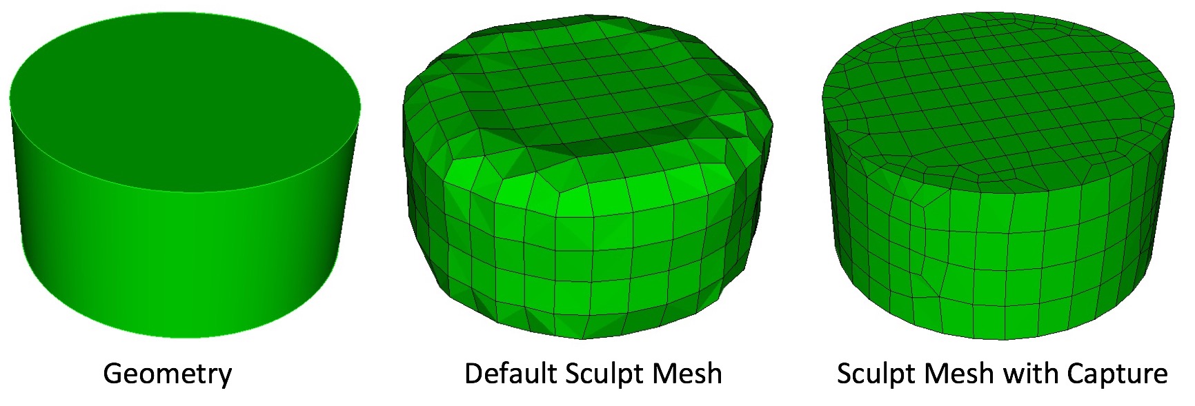
Several options are currently being studied as possible solutions. They include the following:
0 = (off) Capture option is off. No attempt is made at capturing sharp features.
1 = (on) STL geometry is used as basis for feature capture. A user defined feature angle is used (capture_angle) to first generate groups of facets from the STL geometry based on capture_angle. Topological curves are defined based on projections to closest surface facets and edges. With default smoothing option, the surface nodes will be projected to the closest STL surfaces as a final step before exporting the exodus mesh. Consider using smooth = to_geometry option.
2 = (exterior_surfaces) Only exterior surfaces are captured. Uses the same procedure as described in capture = 1, except that interior surfaces (those with two adjacent volumes), will be ignored in the capture and projections stage.
3 = (projections_only) For this option, additional topology based on feature angle is not extracted. Only the final projection of surface nodes to the STL facets is done. Note that this option is useful for organic shapes that do not have sharp features, or where sharp features should be ignored.
4 = (feature_angle_smooth) This option uses the procedure outlined in capture = 1, except that the smooth = to_geometry is used by default. Note that capture = 1 used with smooth = to_geometry should be identical to this option.
5 = (topology_smooth) Curve topology is defined similar to capture = 1, except that element face topology is first determined based on closest assigned facet. Curve topology is then extracted based on adjacent element face associativity. Surface node projections are only done for nodes that have unambiguous neighbor associativity. This provides for a tolerant approach to resolving topology that may result in defeaturing. (i.e. where the STL facet topology may be locally more complex than can be resolved by the prescribed resolution). This option also uses the smooth = to_geometry option as default for smoothing. Also note that capture = 5 it is only currently available for serial execution (j=1)
5.4.11.8.9 Capture Angle
Command: capture_angle Angle at which to split surfaces <beta> |
|
Input file command: capture_angle <arg> |
Command line options: -ca <arg> |
Argument Type: floating point value (0 -> 360) |
Command Description:
This is an experimental option still in development. Feature angle for capture option.
5.4.11.8.10 Capture Side
Command: capture_side Project to facet geometry with surface ID |
|
Input file command: capture_side <arg> |
Command line options: -sc <arg> |
Argument Type: integer > 0 |
Command Description:
Generate or import CAD model into Cubit.
Identify and group selected surfaces into a single sideset with unique ID.
In the Sculpt GUI set the sideset generation option to 4.
Turn on the option: Do not Run Sculpt.
In your working directory edit the input file (.i).
Add the option capture_side = <id> to the input file.
Run sculpt in batch using the input file to control execution.
The result should be a mesh where surface nodes closest to the surfaces identified by the unique sideset ID will lie precisely on their closest surface.
5.4.11.8.11 Defeature
Command: defeature Apply automatic defeaturing |
|
Input file command: defeature <arg> |
Command line options: -df <arg> |
Argument Type: integer (0, 1, 2, 3) |
Input arguments: off (0) |
filter (1) |
collapse (2) |
filter_and_collapse (3) |
Command Description:
off (0): No defeaturing performed (default)
filter (1): Filters the Cartesian grid data so that groupings of cells of a common material with less than min_vol_cells will be reassigned to the predominant neighboring material. If the min_vol_cells argument is not specified, the minimum number of cells in a volume will be set to 5. This has the effect of removing small volumes that would otherwise be generated. This option will also remove protrusions, where a cell surrounded on 4 or 5 sides by another material ID will be reassigned to the predominant neighboring material. This option is available with multiple processors. See also the defeature_iters and defeature_bbox options for additional control of the defeature = filter option. The compare_volume option can also be used to validate that changes made to material volumes are within acceptable limits.
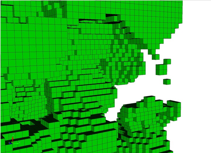
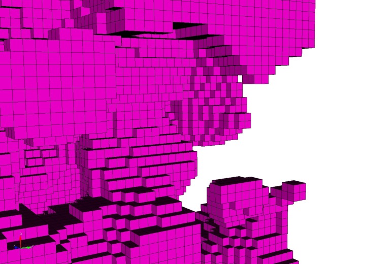
Figure 283: Example grid cells before and after defeaturing has been applied
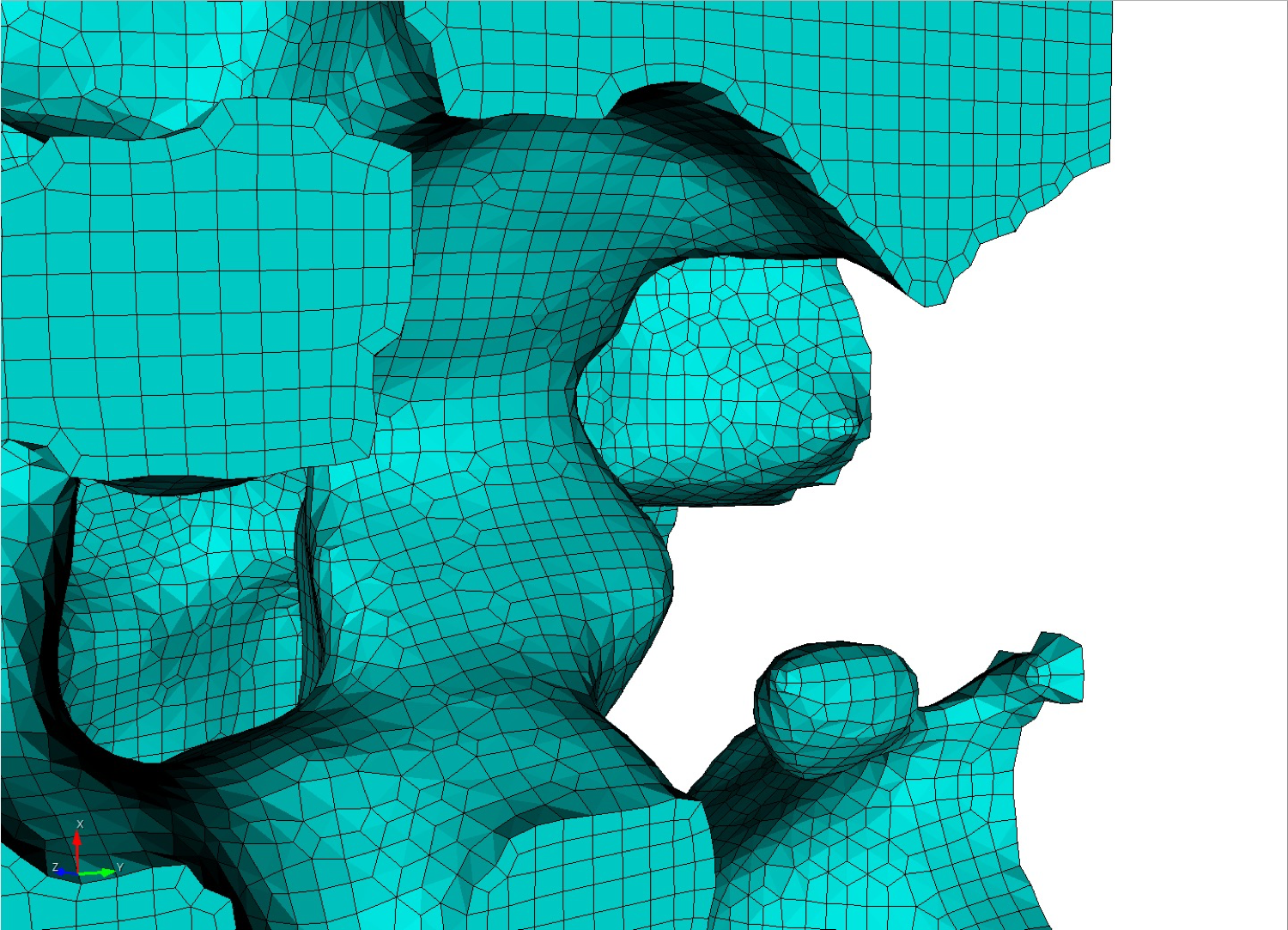
- collapse (2): Curve and surface collapses are performed. This option is only available when used with the trimesh option. After geometry has been extracted and built from the volume fraction data curves containing exactly one mesh edge are collapsed into a single vertex. Surfaces that are identified with exactly 2 curves, each of which have 2 mesh edges are collapsed into a single curve. Only available as serial option (-j 1)
filter_and_collapse (3): Performs both option filter (1) and collapse (2) on a trimesh. Only available as serial option (-j 1)
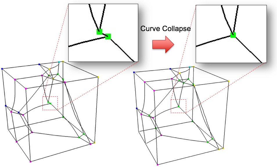
5.4.11.8.12 Minimum Number of Cells in a Volume
Command: min_vol_cells Minimum number of cells in a volume |
|
Input file command: min_vol_cells <arg> |
Command line options: -mvs <arg> |
Argument Type: integer >= 0 |
Command Description:
When used with defeature options filter (1) or filter_and_collapse (3), specifies the minimum number of cells below which a volume will be eliminated. The cells of small volumes will be absorbed into the predominant material of the neighboring cells. If not specified and defeature options filter (1) or filter_and_collapse (3) are used, the min_vol_cells value will be set to 5.
5.4.11.8.13 Defeature at Bounding Box
Command: defeature_bbox Defeature Filtering at Bounding Box |
|
Input file command: defeature_bbox |
Command line options: -dbb |
Command Description:
The defeature_bbox option is used in conjunction with defeature = filter (1). It is used to modify the defeature filter criteria at cells that are immediately adjacent to the Cartesian grid’s domain boundary. It is most effective for microstructure data but can be used with any input format. The defeature = filter (1) option will remove protrusions identified by cells that are surrounded on 4 or 5 sides by another material. For cells that are at the domain boundary, cells will have missing adjacent cells on at least one face. If the defeature_bbox=true option is used, the missing adjacent cells are considered a different material and counted in the 4 or 5 surrounding cells with a different material. In contrast, the defeature_bbox=false option will not count the missing adjacent cells. Using the defeature_bbox=true has the effect of more aggressively modifying cells at the domain boundaries to avoid protrusions. The default for this option is defeature_bbox=false. It will be ignored if defeature = filter (1) is not used.
5.4.11.8.14 Maximum Number of Defeature Iterations
Command: defeature_iters Maximum Number of Defeaturing Iterations |
|
Input file command: defeature_iters <arg> |
Command line options: -dfi <arg> |
Argument Type: integer >=0 |
Command Description:
Used with the defeature option. Controls the maximum number of iterations of defeature filtering that will be performed. Setting this value greater than the default of 10 can be useful for very noisy data where a significant number of iterations will need to be performed to resolve the geometry.
When performing non-manifold resolution, the defeature state of some of the cells may be effected. As a result, the defeaturing and non-manifold resolution procedures are performed in a loop until no further changes can be made. The defeature_iters sets the maximum number of defeature and non-manifold resolution procedures that will be performed. Note that if defeaturing reaches the maximum iteration value without completely resolving all non-manifold conditions, that subsequent sculpt procedures may not succeed. Set this value higher to allow the defeaturing and non-manifold resolution to run to completion. The stair = 1 option can be used to interrogate the model to see where non-manifold conditions may still exist.
5.4.11.8.15 Thicken a material
Command: thicken_material Expand a given material into surrounding cells |
|
Input file command: thicken_material <arg> |
Command line options: -thm <arg> |
Argument Type: integer >= 0 floating point value (0.0->1.0) |
Command Description: Add additional cells at the boundary of a given material. Takes two input values, a material and a volume fraction between 0 and 1. This option is useful for noisy input data that may not form contiguous volumes. Thickening a material may close small gaps making the material continuous. To perform the thicken operation, cells in adjacent materials are removed and reassigned to the indicated material. This option requires both a valid material ID and volume fraction value, where the volume fraction represents the amount of material to be added to each neighboring cell. For example:
thicken material = 1 0.2
thicken_material = 2 0.5
each neighboring cell to material 1 will change approximately 20 percent of its volume to be material 1. Other materials present in the cell will be decreased accordingly to maintain a sum of 1.0 for each cell. Additional material is accumulated in neighboring cells from each adjacent cell it shares with material 1, so that if for example a neighbor cell shares faces with three cells of material 1, it will add 0.6 (0.2 X 3) of material 1 volume fraction to the neighbor. If more than one thicken_material option is used, the thicken operation will be performed in the order they appear in the input. For the above example, material 1 would first be thickened, followed by material 2. If materials 1 and 2 are adjacent, thickening in this case, material 2 would take precedence, potentially removing cells from material 1 at their interface.
Figure 286: Bitmap input is used on a Cartesian base grid to generate the mesh for complex head and brain anatomy. Left: Some of the materials prior to applying the thicken_material option. Right: After applying the thicken_material option.
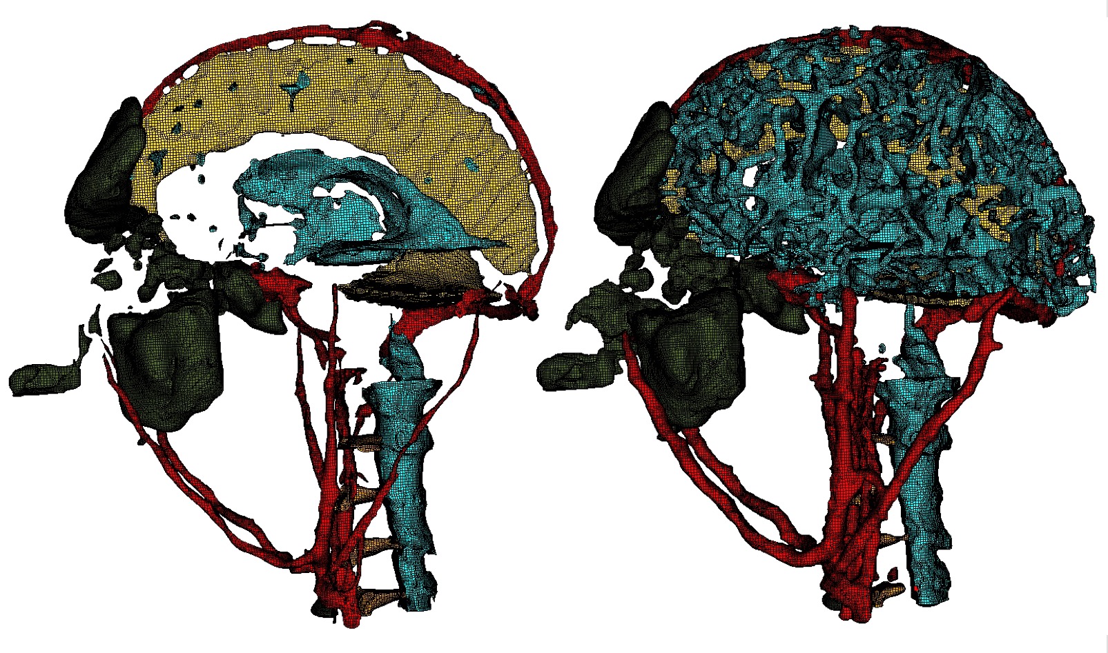
5.4.11.8.16 Insert void material to remove overlap
Command: thicken_void Insert void material to remove overlap |
|
Input file command: thicken_void <arg> |
Command line options: -thv <arg> |
Argument Type: floating point value (0.0->1.0) |
Command Description: Add additional void material when non-void material is detected as touching or immediately adjacent. Takes one input value, a volume fraction normally about 1.0 that indicates the quantity of volume fraction inserted at each node if the input grid where non-void material adjacency is detected. A value of 1.0 indicates void material equal to the volume of one cell will be added at the nodes, reducing the volume fractions of other materials present in adjacent cells. Smaller input values will generate a smaller gap between materials, but can run the risk of materials bleeding into one another.
This option is useful when it is known that non-void materials in the model should not touch, instead should have a gap where they would otherwise touch or overlap. For example:
thicken_void = 1.0
each node where its adjacent cells have two or more non-void materials present will have additional void material added. In this case, if 8 adjacent cells are assumed, a contribution of 1/8 void volume fraction will be added to each adjacent cell to the node. Other materials present in the cells will be decreased accordingly to maintain a sum of 1.0 for each cell.
5.4.11.8.17 Microstructure Expansion
Command: micro_expand Expand Microstructure grid by N layers |
|
Input file command: micro_expand <arg> |
Command line options: -me <arg> |
Argument Type: integer >= 0 |
--input_micro |
--input_cart_exo |
--input_spn |
In some cases the interior material interfaces may intersect the domain boundaries at small acute angles. When this occurs it may be difficult or impossible to achieve computable mesh quality at these intersections. To address this problem, one or more layers of hexes may be added to the Cartesian grid. The volume fractions from cells at the boundary are copied to generate additional layers. This has the effect of increasing the angle of intersection for any material interfaces intersecting the domain boundary. Usualy a value of 1 or 2 is sufficient to sufficiently improve quality.
Note that the resulting mesh in the expanded layers serves only to improve mesh quality and will only duplicate existing data at the boundaries. It may not reflect the actual material structure within the expansion layers.
Figure 287: (a) Initial mesh (b) One expansion layer added (c) Two expansion layers added
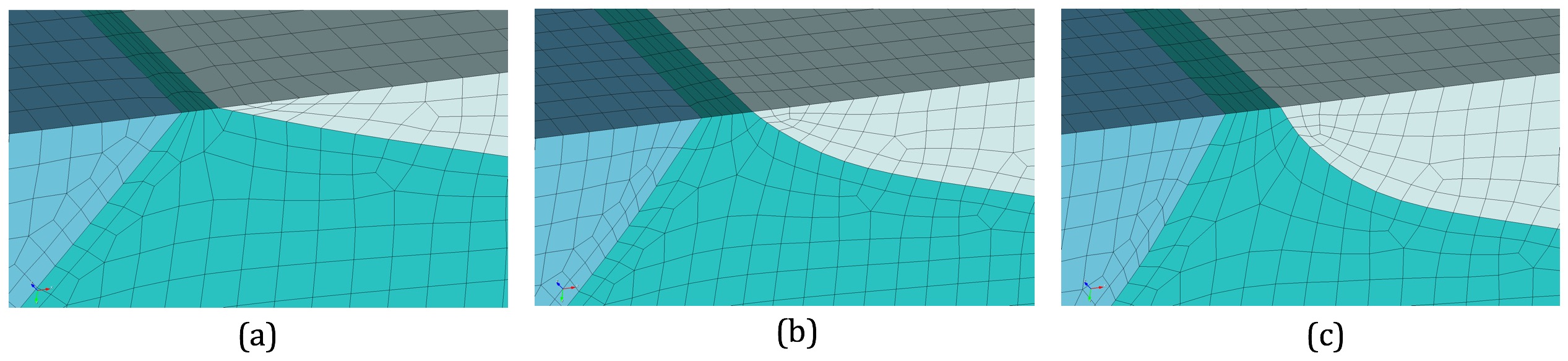
5.4.11.8.18 Microstructure Shave
Command: micro_shave Remove isolated cells at micro. boundaries |
|
Input file command: micro_shave |
Command line options: -ms |
Command Description:
This option potentially modifies the outermost layer of Cartesian cells of a microstructures file. It will identify isolated cells where the assigned material is unique from all of its surrounding cells at the boundary. When this occurs, the cell material is reassigned to the dominant nearby material.
This option is useful if it is noted that a cell structure just barely grazes the exterior planar boundary surface. Poor quality elements can often result with this condition. The micro_shave option will, in effect, remove material from the cell structure, but will result in better quality elements by removing the intersection region with the boundary.
--input_micro |
--input_cart_exo |
--input_spn |
5.4.11.8.19 Remove bad elements below threshold
Command: remove_bad Remove hexes with Scaled Jacobian < threshold |
|
Input file command: remove_bad <arg> |
Command line options: -rb <arg> |
Argument Type: floating point value -1.0 >= 1.0 |
Command Description:
Remove hexes below the specified scaled Jacobian metric.
5.4.11.9 Sculpt Input Data Files
Options for specifying input files to Sculpt. Sculpt uses a method for representing geometry based upon volume fractions defined on a Cartesian or unstructured grid. Sculpt will accept facet-based (STL) or analytic (diatom) geometry, but will first convert the input geometry to the required volume fraction description before generating the hexahedral mesh. Various formats for volume fraction data can also be imported directly into Sculpt and used as the basis for hex meshing. The following formats for geometry are currently supported in Sculpt:
STL (stl_file)
Diatom (diatom_file)
Volume Fractions
Exodus element variables (import_vfrac)
Exodus blocks (import_cart_exo)
Ascii Voxel Data (import_spn)
Ascii Volume Fraction Data (import_micro)
Input Data Files --input -inp |
--stl_file -stl <arg> Input STL file |
--diatom_file -d <arg> Input Diatom description file |
--input_vfrac -ivf <arg> Input from Volume Fraction file base name |
--input_micro -ims <arg> Input from Microstructure file |
--input_cart_exo -ice <arg> Input from Cartesian Exodus file |
--input_spn -isp <arg> Input from Microstructure spn file |
--spn_xyz_order -spo <arg> Ordering of cells in spn file |
--lattice -l <arg> STL Lattice Template File |
5.4.11.9.1 STL File
Command: stl_file Input STL file |
Input file command: stl_file <arg> |
Command line options: -stl <arg> |
Argument Type: file name with path |
Command Description:
File name of a single STL (facet geometry) file to be used as input. Either an stl_file or diatom_file designation should be included to run Sculpt. The stl_file option will support a single STL file. To use multiple STL files, where each file represents a different material, use the diatom_file file option where multiple file names may be specified.
It is recommended that STL files used as input to Sculpt be "water-tight". While in many cases non-watertight geometries will be successful, unexpected or incorrect results may result. It is recommended practice to use Cubit to first import the STL geometry and allow the sculpt parallel command to write a new STL geometry file for use in Sculpt. Cubit’s sculpt parallel command will attempt to stitch and repair any triangle facets that are not completely closed. Other commercial tools are available for STL geometry that may be effective in repairing the geometry prior to use in Sculpt.
5.4.11.9.2 Diatom File
Command: diatom_file Input Diatom description file |
Input file command: diatom_file <arg> |
Command line options: -d <arg> |
Argument Type: file name with path |
Command Description:
File name of a diatom file to be used as input to Sculpt. Both stl_file and diatom_file cannot be used simultaneously. A diatom file is a constructive solid geometry description containing primitives for generating a full geometric definition of the model. Diatoms are commonly used as input to Sandia’s CTH and Alegra codes. Multiple STL files can also be defined in a Diatom file. The following is a simple example of a diatom file that would read 3 different STL files:
diatoms |
package 'blue_material' |
material 1 |
insert stl |
file = 'blue_part1.stl' |
endinsert |
insert stl |
file = 'blue_part2.stl' |
endinsert |
endpackage |
package 'red_material' |
material 2 |
insert stl |
file = 'red_part1.stl' |
endinsert |
endpackage |
enddiatom |
Note that the first two files, blue_part1.stl and blue_part2.stl belong to the same material. As a result, elements generated within the geometry of these files will belong to block 1. Likewise, the elements generated within the geometry of red_part1.stl will belong to block 2.
Bitmap Files
The Diatom format will also support bitmap files. These are binary files that set each cell either on or off for the specified material. The following is an example diatom specification for a bitmap file. Note that the bitmap specification includes nx, ny, nz dimensions for the size of the input file.
diatoms |
package 'Skull' |
material 1 |
insert bitmap |
file = 'skull_bitmap_file' |
nx = 680 |
ny = 408 |
nz = 236 |
endinsert |
endpackage |
enddiatom |
Figure 288: Example mesh generated with Diatom bitmap option
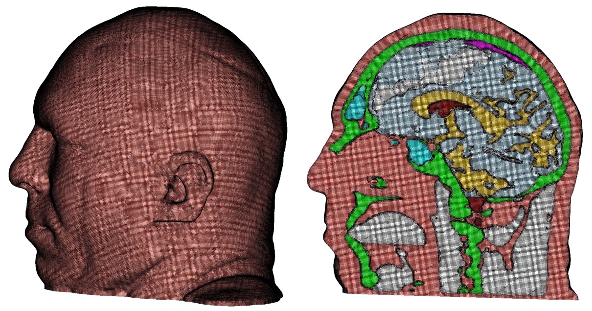
For a full description of the diatom format see the CTH or Alegra documentation.
D. A. Crawford, A. L. Brundage, E. N. Harstad, K. Ruggirello, R. G. Schmitt, S. C. Schumacher and J. S. Simmons, "CTH User’s Manual and Input Instructions, Version 10.3", CTH Development Project, Sandia National Laboratories, Albuquerque, New Mexico 87185, February 14, 2013
5.4.11.9.3 Input Volume Fraction File
Command: input_vfrac Input from Volume Fraction file base name |
Input file command: input_vfrac <arg> |
Command line options: -ivf <arg> |
Argument Type: base file name with path |
Command Description:
Sculpt can optionally take an exodus file containing volume fraction data stored as element variables. Normally the exodus file has initially been written using the –volfrac_file (-vf) option. Since the exodus file will be a Cartesian grid spread across multiple processors, the base filename for the parallel series of exodus files is used as the argument for this command. The input volume fraction file(s) would be used instead of an STL or diatom file. Since computing volume fractions from geometry can be time consuming, precomputing the volume fractions and reading them from a file can be advantageous if multiple meshes are to be generated from the same volume fraction data.
5.4.11.9.4 Input Microstructure File
Command: input_micro Input from Microstructure file |
Input file command: input_micro <arg> |
Command line options: -ims <arg> |
Argument Type: file name with path |
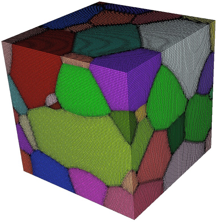
A microstructure file is an ascii text file containing volume fraction data for each cell of a Cartesian grid. The format for this file includes header information followed by data for each cell. The following is an example:
TITLE = triple line system |
VARIABLES = x y z, phi_1, phi_2, phi_3 |
ZONE i = 2 , j = 2 , k = 2 |
0.0000 0.0000 0.0000 0.5000 0.5000 0.0000 |
1.0000 0.0000 0.0000 0.3333 0.3333 0.3334 |
0.0000 1.0000 0.0000 1.0000 0.0000 0.0000 |
1.0000 1.0000 0.0000 0.0000 1.0000 0.0000 |
0.0000 0.0000 1.0000 0.2000 0.4000 0.4000 |
1.0000 0.0000 1.0000 0.6000 0.1000 0.3000 |
0.0000 1.0000 1.0000 0.0000 0.0000 1.0000 |
1.0000 1.0000 1.0000 0.9000 0.0000 0.1000 |
The header information should contain the following:
TITLE: any descriptive character string
VARIABLES: a list of variables separated by spaces or commas. It should include x, y, z as the first three variable names. The remaining names are arbitrary. The number of variable names listed must correspond to the number of data values for each cell of the Cartesian grid.
ZONE: Specify the number of cells in the i, j and k directions (corresponding to x, y, and z respectively)
The body of the file will contain one line per cell of the grid. The first three values correspond to the centroid location of a cell in the grid. The remaining values represent volume fractions for the cell for each variable listed. The sum of the volume fractions for each individual cell should be 1.0.
Currently this format assumes that cell sizes are exactly 1.0 x 1.0 x 1.0 and the minimum cell centroid location is always 0.0, 0.0, 0.0. This results in a Cartesian grid with minimum coordinate = (-0.5, -0.5, -0.5) and maximum coordinate = (i-0.5, j-0.5, k-0.5). If a size other than 1x1x1 is required consider using the scale and/or translate options.
sculpt -j 8 -ims my_micro_file.tec -p 1 |
--smooth 9 (surface smoothing option - no surface projection) --csmooth 2 (curve smoothing option - hermite interpolation) |
--smooth 8 (surface smoothing option - projection to interpolated surface) --csmooth 5 (curve smoothing option - projection to interpolated curve) |
Pillowing: For most 3D models it is recommended using pillowing since triple junctions (curves with at least 3 adjacent materials) will typically be defined where malformed hex elements would otherwise be generated. Surface pillowing (option 1) is usually sufficient to remove poor quality elements at triple junctions.
Figure 290: Pillows (hex layers) inserted at surfaces to improve element quality around curves. Note mesh quality at curve between surfaces A and B.
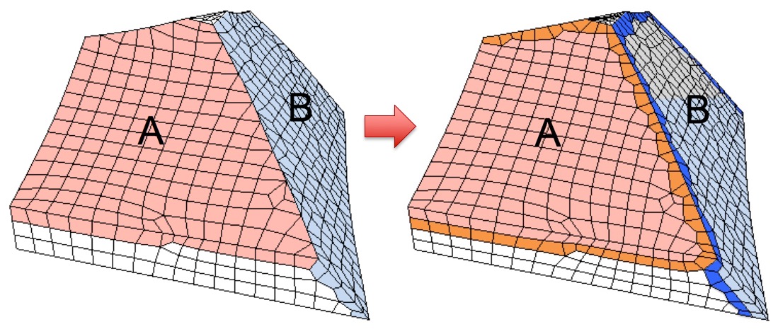
5.4.11.9.5 Input Cartesian Exodus File
Command: input_cart_exo Input from Cartesian Exodus file |
Input file command: input_cart_exo <arg> |
Command line options: -ice <arg> |
Argument Type: file name with path |
Command Description: An exodus mesh containing a Cartesian grid of elements can also be used as the source of a sculpt mesh. For this option the following conditions must be met:
Figure 291: Example Cartesian Exodus file and the resulting hex mesh.
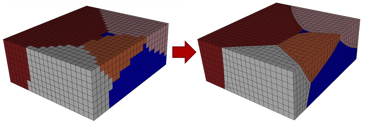
A single (non-parallel) exodus II format file.
Contains only hex elements configured as a Cartesian grid.
All hex elements must be exactly equilateral cubes.
Each hex element has been assigned to exactly one block. (Any number of blocks may be defined in the file)
Provided these conditions are met, sculpt will treat each block as a separate material and generate a smooth conforming mesh between the materials. This option is useful for converting a stair-step mesh into a smooth conforming mesh. The resulting sculpt mesh will have the same dimensions as the original exodus mesh, but will add layers of hexes at material interfaces.
sculpt -j 8 -ice my_cartesian_file.e -p 1 |
--smooth 9 (surface smoothing option - no surface projection) --csmooth 2 (curve smoothing option - hermite interpolation) |
--smooth 8 (surface smoothing option - projection to interpolated surface) --csmooth 5 (curve smoothing option - projection to interpolated curve) |
Pillowing: For most 3D models it is recommended using pillowing since triple junctions (curves with at least 3 adjacent materials) will typically be defined where malformed hex elements would otherwise be generated. Surface pillowing (option 1) is usually sufficient to remove poor quality elements at triple junctions.
5.4.11.9.6 Input Microstructure SPN File
Command: input_spn Input from Microstructure spn file |
Input file command: input_spn <arg> |
Command line options: -isp <arg> |
Argument Type: file name with path |
Command Description:
A .spn file is an optional method for importing volume fraction data into sculpt for meshing. This format is a simple ascii text file containing one integer per cell of a Cartesian grid. Each integer represents a unique material identifier. Any number of materials may be used, however for practical purposes, the number of unique materials should not exceed more than about 50 for reasonable performance.
1 1 2 1 2 1 1 1 1 |
1 2 2 1 2 2 1 1 2 |
2 1 1 1 2 1 1 2 2 |
sculpt -j 8 -x 10 -y 24 -z 15 -isp "my_spn_file.spn" -p 1 |
for (i=0; i<nx; i++) |
for (j=0; j<ny; j++) |
for (k=0; k<nz; k++) |
// read next value from file |
Where nx, ny, nz are the number of cells in each Cartesian direction. This ordering can be changed to nz, ny, nx using the spn_xyz_order option. The initial size of the Cartesian grid will be exactly nx X ny X nz with the minimum coordinate at (0.0, 0.0, 0.0). If a size other than the default is required, consider using the scale and/or translate options.
--smooth 9 (surface smoothing option - no surface projection) --csmooth 2 (curve smoothing option - hermite interpolation) |
--smooth 8 (surface smoothing option - projection to interpolated surface) |
--csmooth 5 (curve smoothing option - projection to interpolated curve) |
Pillowing: For most 3D models it is recommended using pillowing since triple junctions (curves with at least 3 adjacent materials) will typically be defined where malformed hex elements would otherwise be generated. Surface pillowing (option 1) is usually sufficient to remove poor quality elements at triple junctions.
5.4.11.9.7 XYZ ordering of cells in SPN File
Command: spn_xyz_order Ordering of cells in spn file |
Input file command: spn_xyz_order <arg> |
Command line options: -spo <arg> |
Argument Type: integer (0 to 5) |
Input arguments: xyz (0) |
xzy (1) |
yxz (2) |
yzx (3) |
zxy (4) |
zyx (5) |
Command Description:
for (i=0; i<nx; i++) |
for (j=0; j<ny; j++) |
for (k=0; k<nz; k++) |
// read next value from file |
If the spn file has the cells in a different order, use this option to specify the order. 0 (xyz) is the default.
5.4.11.9.8 STL Lattice Template File
Command: lattice STL Lattice Template File |
Input file command: lattice <arg> |
Command line options: -l <arg> |
Argument Type: file name with path |
Command Description:
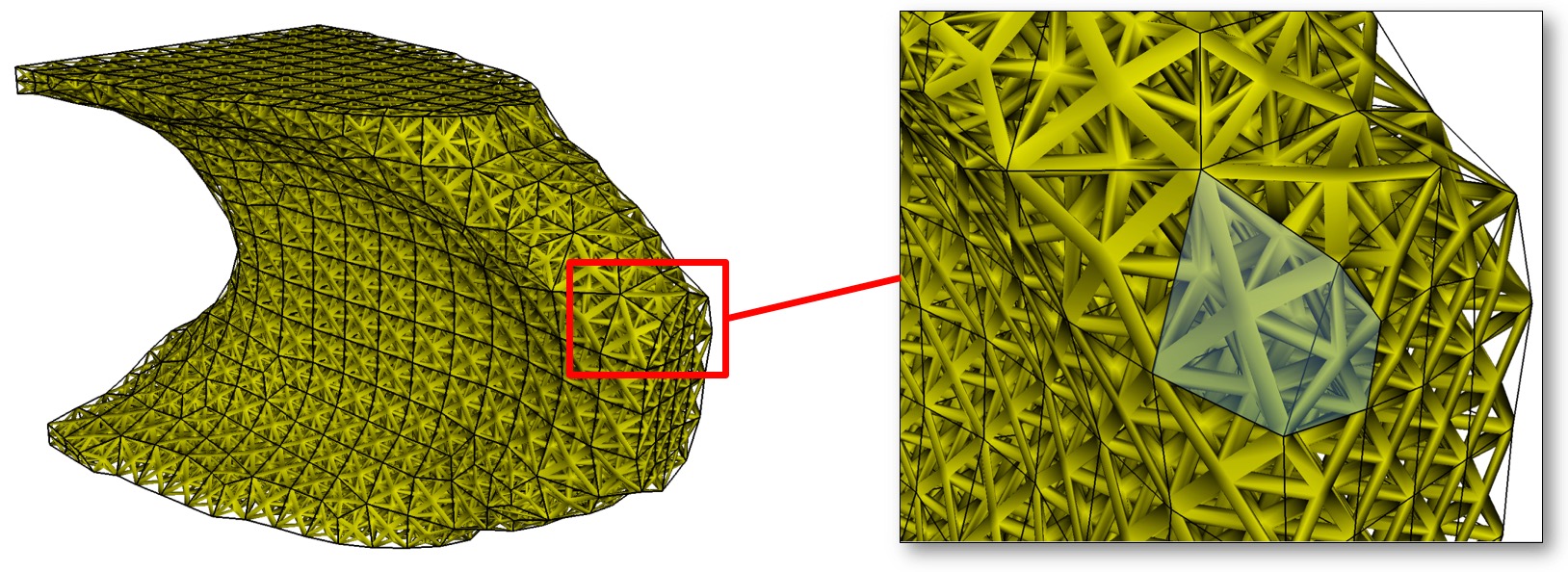
Generate a lattice structure from a hex mesh. This command takes the name of an STL format template file which defines the lattice over a unit cube. To generate a valid lattice structure, the facets should be symmetric to the three coordinate planes. The lattice structure will be transformed and copied into each hex of the mesh. The result will be an STL file containing lattice geometry for the mesh.
This option currently requires the name of an exodus mesh on which to define the lattice. Use the –exodus_file (-e) option to specify its path. The current implementation is limited to one block, however if a second block is contained in the Exodus file it will be treated as a solid and stl facets will be generated at the skin of the block.
The name of the output STL file may also be defined by using the –stl_file (-stl) option. If no stl file is specified, the output will use the name of the input exodus file with the extension "_lattice.stl" appended.
In addition to the full lattice geometry, an additional file containing only the lattice from the first layer of hexes will be written. This may be useful in reducing the size of the STL file for visualization purposes only. The name of this file will be the name of the full STL geometry file with the extension ".vis.stl" appended.
BEGIN SCULPT |
lattice = lattice_template.stl $contains unit cube with triangles |
exodus_file = file.e $ hex mesh containing one or two element blocks |
stl_file = file.stl $ name of output stl file |
END SCULPT |
Note that this option is currently limited to serial execution (-j 1)
5.4.11.10 Sculpt Mesh Type
Sculpt options for specifying the type of mesh that will be generated. The default mesh type that will be produced from Sculpt is an unstructured all-hex mesh that will attempt to conform as closely as possible to the input geometry. Sculpt will normally generate its mesh on the interior of the input geometry, however with the mesh_void option, it can also generate the mesh on the exterior of the geometry, out to the extent of the user-defined Cartesian overlay grid.
In addition to the default hex mesh, other types of meshes may be produced. This includes the stair-step mesh where the cells of the Cartesian grid inside or intersecting the geometry are used directly as the mesh without projections or smoothing. A triangle mesh may also be generated, which can be used as the basis for a facet-based geometry representation. Other methods include the capabilities to generate a hex-dominant mesh with hexes and tets as well as the ability to include degenerate elements.
Mesh Type --type -typ |
--stair -str <arg> Generate Stair-step mesh |
--mesh_void -V <arg> Mesh void |
--trimesh -tri Generate tri mesh of geometry surfaces |
--tetmesh -tet <arg> Under Development |
--deg_threshold -dg <arg> Convert hexes below threshold to degenerates |
--max_deg_iters -dgi <arg> Maximum number of degenerate iterations |
--htet -ht <arg> Convert hexes below quality threshold to tets |
--htet_method -hti <arg> Method used for splitting hexes to tets |
--htet_material -htm <arg> Convert hexes in given materials to tets |
--htet_transition -htt <arg> Transition method between hexes and tets |
--htet_pyramid -htp <arg> Local transition pyramid |
--htet_tied_contact -htc <arg> Local transition tied contact |
--htet_no_interface -htn <arg> Local transition none |
5.4.11.10.1 Stair
Command: stair Generate Stair-step mesh |
|
Input file command: stair <arg> |
Command line options: -str <arg> |
Argument Type: integer (0, 1, 2, 3) |
Input arguments: none (0) |
off (0) |
on (1) |
full (1) |
interior (2) |
fast (3) |
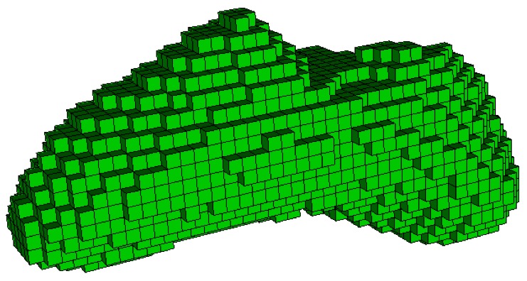
The stair option generates a stair-step mesh where the cells of the Cartesian grid are used in the final mesh without projection or smoothing to the material interfaces. Cells selected from the Cartesian grid to be used in the final mesh will have volume fraction greater than 0.5. Several different options for the stair argument are available:
off (0): Stair option is off (default)
full (1): Stair-step mesh is generated, but additional processing is done to ensure material interfaces are manifold. This option may add or subtract cells from the basic mesh (where volume fraction > 0.5) to ensure no non-manifold connections between nodes and edges exist in the final mesh.
interior (2): The exterior boundary will be smooth while internal material interfaces will be stair-step. This option also ensures manifold connections between elements.
fast (3): Generates the final mesh based only on volume fraction criteria. No additional processing is done to ensure manifold connections between edges and nodes.
5.4.11.10.2 Mesh Void
Command: mesh_void Mesh void |
|
Input file command: mesh_void <arg> |
Command line options: -V <arg> |
Argument Type: true/false or only |
Input arguments: off (0) |
false (0) |
on (1) |
true (1) |
only (2) |
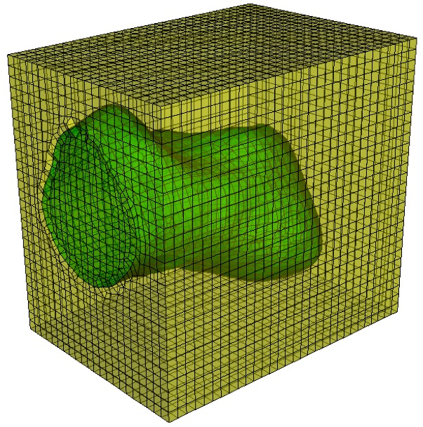
The mesh_void accepts the following parameters:
off (0): No mesh is generated in the void region
on (1): Mesh is generated in the void region
only (2): Mesh is generated only in the void region and not in the material
If mesh_void option is set to on or only, then the void space surrounding the geometry will be treated as a separate material. Elements will be generated in the void to the extent of the Cartesian grid boundaries. If void_mat option is not used, the material ID of elements in the void region will be the maximum material ID in the model + 1. See also the separate_void_blocks option to separate the void elements into contiguous blocks.
5.4.11.10.3 Trimesh
Command: trimesh Generate tri mesh of geometry surfaces |
|
Input file command: trimesh |
Command line options: -tri |
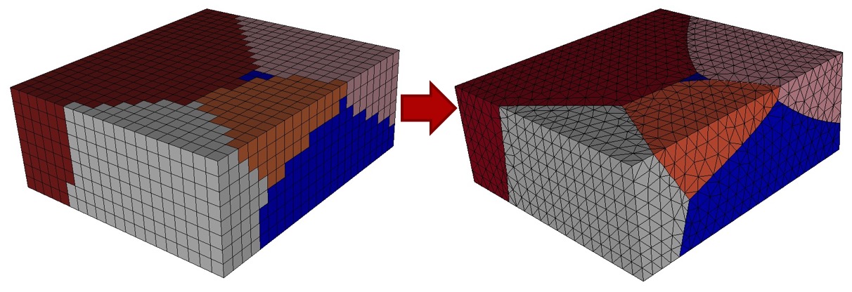
Generate a triangle mesh of the surface geometry. Surface geometry will be defined based on input grid resolution as well as user defined smoothing smoothing parameters. Resulting exodus mesh will contain only TRI elements. All TRI elements will be assigned to the same block in the exodus file.
import s2g <root filename> |
5.4.11.10.4 Tetmesh
Command: tetmesh Under Development |
|
Input file command: tetmesh <arg> |
Command line options: -tet <arg> |
Argument Type: none |
Input arguments: off (0) |
on (1) |
true (1) |
meshgems (2) |
The meshgems (2) option uses a third party tet mesher to place interior tets. Triangle mesh is defined by splitting quads on surface. Both tetmesh options are currently only implemented for serial execution.
5.4.11.10.5 Degenerate (Edge Collapse) Threshold
Command: deg_threshold Convert hexes below threshold to degenerates |
|
Input file command: deg_threshold <arg> |
Command line options: -dg <arg> |
Argument Type: floating point value (-1.0 -> 1.0) |
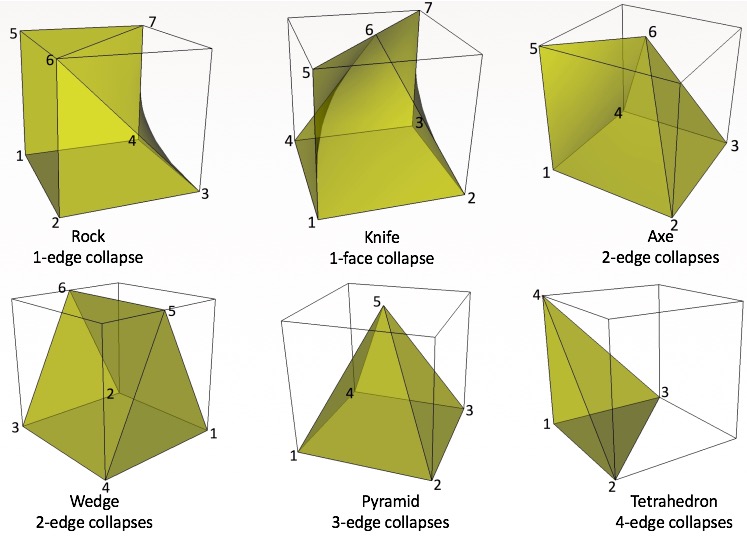
Some geometries will not permit a usable mesh with a traditional all-hex mesh. Sculpt includes the option to automatically and selectively collapse element edges to improve low-quality elements. The max_deg_iters and the deg_threshold values are used to control the creation of degenerates. Degenerate elements are treated as standard hex elements, but use repeated nodes in the eight-node connectivity array.
The deg_threshold value indicates scaled Jacobian threshold for edge collapses. Nodes at hexes below this threshold will be candidates for edge collapses, provided doing so will improve the minimum scaled Jacobian at the neighboring hexes. Default is -1.0.
5.4.11.10.6 Maxmimum Degenerate Iterations
Command: max_deg_iters Maximum number of degenerate iterations |
|
Input file command: max_deg_iters <arg> |
Command line options: -dgi <arg> |
Argument Type: integer >= 0 |
Maximum number of edge collapse iterations to perform to create degenerate hex elements. Default is 0. See also deg_threshold
5.4.11.10.7 HTet
Command: htet Convert hexes below quality threshold to tets |
|
Input file command: htet <arg> |
Command line options: -ht <arg> |
Argument Type: floating point value (-1.0 -> 1.0) |
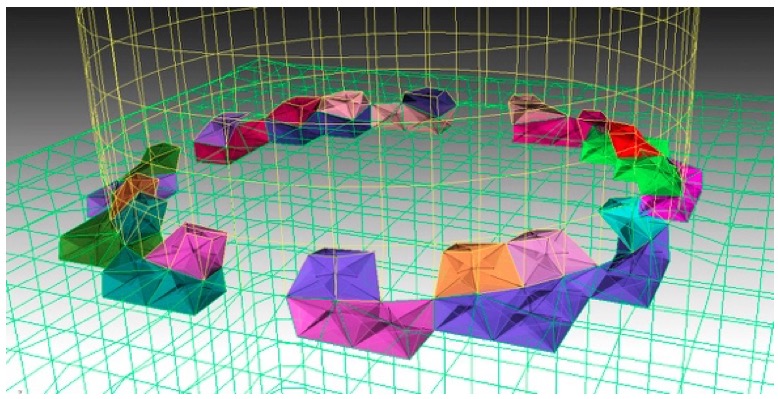
Automatically generate tets in place of poor quality elements. This option can be used to eliminate poor quality hex elements by replacing each hex that falls below the user defined Scaled Jacobian with 6 or 24 tets. The method used for splitting is controlled by the htet_method option. The default threshold value for htet is -1.0, which turns off the generation of all tets. A value of 1.0 will split all hexes into tets.
If a neighboring element is a hex, and will not be split, one may choose whether to use pyramid transitions or have hanging nodes. The default is to have hanging nodes with a tied contact condition being created. The transition type may be specified with the htet_transition command.
If tet blocks are created, their ids will be the material id plus an offset based on the maximum material id. Likewise, any pyramid blocks created will be offset as well, with their ids coming after hex block ids if there are no tets, or with their ids coming after tet blocks.
5.4.11.10.8 HTet Method
Command: htet_method Method used for splitting hexes to tets |
|
Input file command: htet_method <arg> |
Command line options: -hti <arg> |
Argument Type: integer (1, 2) |
Input arguments: none (0) |
structured (1) |
unstructured (2) |
Command Description:
Specifies which method is used for splitting hexes into tets:
structured (0): Each hex is subdivided into 24 tets. Additional nodes are The 24 tets are formed by inserting one node at the center of each face and one on the interior.
unstructured (1): Each hex is subdivided into 6 tets. No additional nodes are inserted. Note that the unstructured method does not currently support the htet_transition options pyramid and tied_contact.
Default htet_method is structured (0).
5.4.11.10.9 HTet Material
Command: htet_material Convert hexes in given materials to tets |
|
Input file command: htet_material <arg> |
Command line options: -htm <arg> |
Argument Type: integer >= 0 |
Command Description:
Generate tets in place hexes in a given material. This option can be given multiple times to specify multiple materials. Each hex in a material is replaced with 24 tets. The 24 tets are formed by inserting one node at the center of each face and one on the interior.
If an neighboring element is a hex, and will not be split, one may choose whether to use pyramid transitions or have hanging nodes. The default is to have hanging nodes with a tied contact condition being created. The transition type may be specified with the htet_transition command.
If tet blocks are created, their ids will be the material id plus an offset based on the maximum material id. Likewise, any pyramid blocks created will be offset as well, with their ids coming after hex block ids if there are no tets, or with their ids coming after tet blocks.
htet_material = 10 |
htet_material = 12 |
htet_transition = pyramid |
htet_no_interface = 10 13 |
Figure 298: Simple example of the use of hybrid tet-hex capability using the above example input. Materials 10 and 12 use tet elements while 13 remains hexes. The default transition is to use pyramids, while the specific interface between 10 and 13 has no interface.
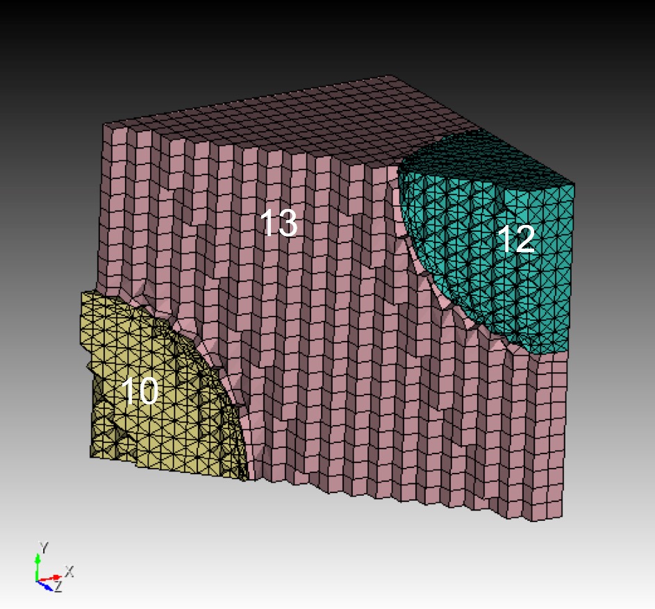
5.4.11.10.10 HTet Transition
Command: htet_transition Transition method between hexes and tets |
|
Input file command: htet_transition <arg> |
Command line options: -htt <arg> |
Argument Type: none/pyramid/tied_contact |
Input arguments: none (0) |
pyramid (1) |
tied_contact (2) |
Command Description:
When generating tets adjacent to hexes, the transition type between the two elements can be defined. Possible options are:
none (0): No transition between hex and tet
pyramid (1): Pyramid transition between hex and tet
tied_contact (2): Tied contact condition between hex and tet
If pyramid transition is specified, the hex may be split into 1 pyramids and 20 tets, 2 pyramids and 16 tets, 3 pyramids and 12 tets, and so forth. The mesh will remain conformal if pyramid transition is specified.
A tied contact condition can be defined to ensure continuity of the neighboring tets and hexes. To facilitate this, one additional nodeset and sideset will be generated and output to the exodus file if the gen_sidesets = variable (2) option is specified. The sideset and nodeset will be identified with the following IDs:
Sideset 10000 = the set of hex faces that interface a set of 4 tets.
Nodeset 1000 = the set of nodes at the interface between hexes and tets. One node per face in Sideset 10000 will be included.
5.4.11.10.11 Local HTet Transition Pyramid
Command: htet_pyramid Local transition pyramid |
|
Input file command: htet_pyramid <arg> |
Command line options: -htp <arg> |
Argument Type: integer(s) >= 0 |
Command Description:
When generating tets adjacent to hexes, pyramid transitions can be specified for a given material or material interface. To specify a material interface, two material ids are given to specify pyramid transition between the two materials. To specify multiple materials or multiple material interfaces, this command may be used multiple times.
5.4.11.10.12 Local HTet Transition Tied Contact
Command: htet_tied_contact Local transition tied contact |
|
Input file command: htet_tied_contact <arg> |
Command line options: -htc <arg> |
Argument Type: integer(s) >= 0 |
Command Description:
When generating tets adjacent to hexes, tied contact transitions can be specified for a given material or material interface. To specify a material interface, two material ids are given to specify tied contact transition between the two materials. To specify multiple materials or multiple material interfaces, this command may be used multiple times.
5.4.11.10.13 Local HTet Transition None
Command: htet_no_interface Local transition none |
|
Input file command: htet_no_interface <arg> |
Command line options: -htn <arg> |
Argument Type: integer(s) >= 0 |
Command Description:
When generating tets adjacent to hexes, no transition can be specified for a given material or material interface. To specify a material interface, two material ids are given to specify no transition between the two materials. To specify multiple materials or multiple material interfaces, this command may be used multiple times.
5.4.11.11 Sculpt Output
Sculpt options for specifying output. The primary format for the hex meshes produced from Sculpt is Exodus II. One exodus file will be produced for each processor based upon the -j or num_procs argument. If required, the exodus files can be joined using the epu utility.
Output --output -out |
--exodus_file -e <arg> Output Exodus file base name |
--volfrac_file -vf <arg> Output Volume Fraction file base name |
--quality -Q Dump quality metrics to file |
--export_comm_maps -C Export parallel comm maps to debug exo files |
--write_geom -G Write geometry associativity file |
--write_mbg -M Write mesh based geometry file <beta> |
--compare_volume -cv Report vfrac and mesh volume comparison |
--compute_ss_stats -css Report sideset statistics |
5.4.11.11.1 Exodus File
Command: exodus_file Output Exodus file base name |
Input file command: exodus_file <arg> |
Command line options: -e <arg> |
Argument Type: character string |
Command Description:
model.e.3.0 |
model.e.3.1 |
model.e.3.2 |
model_diatom_results.e.3.0 |
model_diatom_results.e.3.1 |
model_diatom_results.e.3.2 |
A full path may be used when specifying the base exodus file name, otherwise files will be placed in the current working directory. If the exodus_file option is not used, exodus files will be placed in the same directory as the input diatom or stl file.
5.4.11.11.2 Volume Fraction File
Command: volfrac_file Output Volume Fraction file base name |
Input file command: volfrac_file <arg> |
Command line options: -vf <arg> |
Argument Type: character string |
Command Description:
Optionally generate exodus files containing a hex mesh of the Cartesian grid containing volume fraction data as element variables. This series of parallel exodus files can later be used as direct input to sculpt using the –input_vfrac (-ivf) command. If not specified, no volume fraction data files will be generated.
5.4.11.11.3 Quality
Command: quality Dump quality metrics to file |
Input file command: quality |
Command line options: -Q |
Command Description:
A file named ’quality.csv’ will be created in the current working directory (or appended). Quality metrics and other details of the run will be written to this file. This option is currently off by default.
5.4.11.11.4 Export Communication Maps
Command: export_comm_maps Export parallel comm maps to debug exo files |
Input file command: export_comm_maps |
Command line options: -C |
Command Description:
Used for debugging and verification. Exodus files of the mesh containing the communication nodes and faces at processor boundaries will be written as nodes and side sets. This provides a way to visually check the validity of the parallel communication maps.
5.4.11.11.5 Write S2G Geometry File
Command: write_geom Write geometry associativity file |
Input file command: write_geom |
Command line options: -G |
Command Description:
An s2g (Sculpt to Geometry) file, with the pattern <fileroot>.s2g, will be produced when this argument is used where fileroot is the string specified by the –exodus_file or -e option. An s2g file includes geometry associativity for the exodus file that is written. If used with Cubit’s "import s2g <fileroot>" a mesh-based geometry will be generated in Cubit with geometric entities prescribed by Sculpt through the s2g file.
When used with the –trimesh option, the s2g file can provide information to Cubit to build a set of mesh-based geometry volumes where only the surfaces are meshed. This is useful for using the tet meshing capabilities in Cubit to mesh the discrete geometry that was generated in Sculpt. For example, a tet mesh may be constructed from microstructures spn data (see import_spn) with the following workflow:
- Run Sculpt to generate an exodus and s2g file. An example input file may look like the following:
begin sculpt
import_spn = myfile.spn
trimesh = true
write_geom = true
pillow = 1
end sculpt
- Import the file into Cubit to generate a mesh based geometry:
import s2g myfile
- Delete the triangle mesh, set sizes and mesh:
delete mesh
vol all scheme tetmesh
vol all size 2.0
mesh vol all
Note that the write_geom and trimesh options are still in development and will currently only work with a single processor (-j 1).
5.4.11.11.6 Write Mesh Based Geometry
Command: write_mbg Write mesh based geometry file <beta> |
Input file command: write_mbg |
Command line options: -M |
Command Description:
An MBG (Mesh Based Geometry) file will be produced when this argument is used with the pattern <fileroot>.mbg, where fileroot is the string specified by the –exodus_file or -e option. An MBG file includes the surface and topology definition defined by sculpt as a result of the interface reconstruction process. It will correspond to the boundary of the 3D elements that are generated in the exodus file, or the surface elements generated with the –trimesh option.
import mbg "<fileroot>.mbg" |
5.4.11.11.7 Report VFrac to Mesh Volume Comparison
Command: compare_volume Report vfrac and mesh volume comparison |
Input file command: compare_volume |
Command line options: -cv |
Command Description:
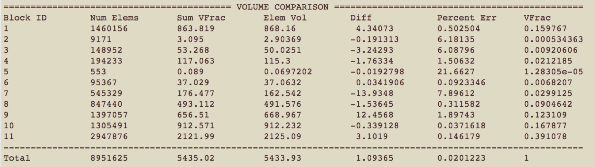
The following is a brief description of each column:
Block ID: ID of material/block
Num Elems: Number of hex elements assigned to block in final mesh
Sum VFrac: Sum of input volume fraction for block. For STL or diatom geometry, approximates the volume fraction. For 3D image data (ie. bitmap, input_spn) sums the exact volume fraction input.
Elem Vol: Sum of final mesh volume for block
Diff: Absolute difference between input and output volume fractions for block. (Elem Vol - Sum VFrac)
Percent Err: Percent error represented by Difference between input and output volume fractions for block
VFrac: Total volume fraction represented by Elem Vol. for block. VFrac volume should sum to 1.0.
5.4.11.11.8 Report Sideset Statistics
Command: compute_ss_stats Report sideset statistics |
Input file command: compute_ss_stats |
Command line options: -css |
Command Description:
A report will be generated and printed to the terminal following the mesh summary that displays the statitics for the surface areas of the sidesets in the final FEA mesh. This is often useful for microstructures use cases where it may be important to know the interface area between materials. This should be used with the gen_sidesets option to be effective.
5.4.11.12 Sculpt Process Control
Options for controlling the execution of Sculpt. Sculpt is a parallel application that uses MPI to distribute and build the hex mesh on multiple processors. The -j or num_procs option is normally used to specify the number of processors to use. Sculpt will write a separate exodus file for each processor, which can be joined into a single file using the epu utility. While any number of processors may be used, you would normally use a -j value less than or equal to the number of cores available on your hardware.
Process Control --process -pc |
--num_procs -j <arg> Number of processors requested |
--input_file -i <arg> File containing user input data |
--debug_processor -D <arg> Sleep to attach to processor for debug |
--debug_flag -dbf <arg> Dump debug info based on flag |
--quiet -qt Suppress output |
--print_input -pi Print input values and defaults then stop |
--version -vs Print version number and exit |
--threads_process -tpp <arg> Number of threads per process |
--iproc -ip <arg> Number of processors in I direction |
--jproc -jp <arg> Number of processors in J direction |
--kproc -kp <arg> Number of processors in K direction |
--periodic -per Generate periodic mesh |
--check_periodic -cp <arg> Check for periodic geometry |
--check_periodic_tol -cpt <arg> Tolerance for checking periodicity |
--periodic_axis -pax <arg> Axis periodicity is about |
--periodic_nodesets -pns <arg> Nodesets ids of master/slave nodesets |
--build_ghosts -bg Write ghost layers to exodus files for debug |
--vfrac_method -vm <arg> Set method for computing volume fractions |
5.4.11.12.1 Number of Processors
Command: num_procs Number of processors requested |
Input file command: num_procs <arg> |
Command line options: -j <arg> |
Argument Type: integer > 0 |
Command Description:
The number of processors that Sculpt will use to generate the mesh. For a structured, Cartesian base grid, the domain will be automatically divided into roughly equal sized rectangular regions based on this value. For unstructured input (see –input_mesh), to utilize more than one processor, the base mesh must first be docomposed into the same number of regions specified by num_procs. The decomp tool, part of the Sandia, SEACAS tool suite can be used to break up an exodus mesh into multiple regions suitable for sculpt input. An independent mesh of a portion of the domain is generated on each processor. Continuity across processor boundaries is maintained with MPI (Message Passing Interface). Each processor will write a separate Exodus II file to disk containing its portion of the domain. The Sandia SEACAS tool, epu can be used to join parallel files into a single file if desired.
If not specified on the command line, the number of processors used will be 1.
For additional control on the arrangement of processor domains on a Cartesian base grid, see arguments iproc, jproc, kproc.
5.4.11.12.2 Input File
Command: input_file File containing user input data |
Input file command: input_file <arg> |
Command line options: -i <arg> |
Argument Type: file name with path |
Command Description:
Rather than specifying a complicated series of arguments on the command line, an input file may also be used. An input file is a simple text file containing all arguments and parameters to be used in the current sculpt run. Input files are normally expected to have a ".i" extension. Arguments used in the input file are limited to the Long Names indicated for each command.
BEGIN SCULPT |
stl_file = "mygeom.stl" |
cell_size = 0.5 |
exodus_file = "mymesh" |
mesh_void = true |
END SCULPT |
sculpt -j 4 -i myinput.i |
Note that the number of processors (-j) should always be used on the command line and cannot be included in the input file. Relative or absolute paths for files may also be used.
5.4.11.12.3 Debug Processor
Command: debug_processor Sleep to attach to processor for debug |
Input file command: debug_processor <arg> |
Command line options: -D <arg> |
Argument Type: integer >= 0 |
Command Description:
Used for debugging. All processes will sleep until the designated process is attached to a debugger. Note: value of 0 corresponds to first processor, 1 to second, etc.
5.4.11.12.4 Debug Flag
Command: debug_flag Dump debug info based on flag |
Input file command: debug_flag <arg> |
Command line options: -dbf <arg> |
Argument Type: integer >= 0 |
Input arguments: off (0) |
lost_nodes (1) |
non-manifold (2) |
defeature (3) |
thickening (4) |
initial-projections (5) |
reversal (6) |
gq-color (8) |
gq-full (9) |
hostname (10) |
Command Description:
Used for debugging. Set flag to dump specific info based on the following:
0 (off) Default, No debug output
1 (lost_nodes) Dump processor lost node info
2 (non-manifold) Export Non-manifold resolution state as exodus file after each inner and outer iteration.
3 (defeature) Export Defeature state as exodus file after each inner and outer iteration.
4 (thickening) Export the Thickened state as exodus file after each material has been thickened.
Guaranteed Quality:
5 (initial-projections) Turn off initial minimizer projection.
6 (reversal) Use Non-manifold reversal case
7 Combine debug_flag 5 and 6
8 (gq-color) Use guaranteed quality laplacian color smoothing
9 (gq-full) Combine debug_flags 5,6 and 8
10 (hostname) Display the host name for each processor
5.4.11.12.5 Quiet
Command: quiet Suppress output |
Input file command: quiet |
Command line options: -qt |
Command Description:
Suppress any output to the command line from Sculpt as it is running.
5.4.11.12.6 Print Input
Command: print_input Print input values and defaults then stop |
Input file command: print_input |
Command line options: -pi |
Command Description:
Display all input parameters and defaults used in the current Sculpt run to the output window and then stop. No mesh (or volume fractions) will be generated.
5.4.11.12.7 Version
Command: version Print version number and exit |
Input file command: version |
Command line options: -vs |
Command Description:
Prints Sculpt version information and exits.
5.4.11.12.8 Threads Per Processor
Command: threads_process Number of threads per process |
Input file command: threads_process <arg> |
Command line options: -tpp <arg> |
Argument Type: integer > 0 |
Command Description:
This option is currently experimental and under development. Sculpt may use shared memory parallelism to improve performance. When built with the Kokkos library, some algorithms in sculpt will use shared memory parallel threads in addition to MPI distributed memory parallelism (MPI+X). Currently this option is implemented only for surface and volume Laplacian smoothing algorithms. This option may not be available requiring a custom build of sculpt to be used. Check with developers if you would like to use this option.
5.4.11.12.9 Number of processors in I
Command: iproc Number of processors in I direction |
Input file command: iproc <arg> |
Command line options: -ip <arg> |
Argument Type: integer > 0 |
Command Description:
Arguments iproc, jproc and kproc provide user control over the processor decomposition in I, J, and K directions respectively. iproc * jproc * kproc must equal the number of processors specified on the command line using the -j option.
5.4.11.12.10 Number of processors in J
Command: jproc Number of processors in J direction |
Input file command: jproc <arg> |
Command line options: -jp <arg> |
Argument Type: integer > 0 |
Command Description:
Arguments iproc, jproc and kproc provide user control over the processor decomposition in I, J, and K directions respectively. iproc * jproc * kproc must equal the number of processors specified on the command line using the -j option.
5.4.11.12.11 Number of processors in K
Command: kproc Number of processors in K direction |
Input file command: kproc <arg> |
Command line options: -kp <arg> |
Argument Type: integer > 0 |
Command Description:
Arguments iproc, jproc and kproc provide user control over the processor decomposition in I, J, and K directions respectively. iproc * jproc * kproc must equal the number of processors specified on the command line using the -j option.
5.4.11.12.12 Generate Periodic Mesh
Command: periodic Generate periodic mesh |
Input file command: periodic |
Command line options: -per |
Command Description:
Generates a periodic mesh for either Cartesian or unstructured mesh input. Ensures that resulting mesh nodes and faces are precisely matching on opposite sides of the mesh.
BEGIN SCULPT |
diatom_file = geometry_file.diatom |
input_mesh = input_exodus_file.g |
exodus_file = output_exodus_file |
smooth = to_geometry |
capture = 5 |
capture_angle = 10 |
free_surface_sideset = 1000 |
gen_sidesets = input_mesh_and_free_surfaces |
periodic = true |
periodic_nodesets = 3224 3225 |
periodic_axis = 0 0 0 0 1 0 |
END SCULPT |
BEGIN SCULPT |
diatom_file = spheres_periodic.diatom |
xmin = -18.705510 |
ymin = -18.705510 |
zmin = -18.705510 |
xmax = 18.705510 |
ymax = 18.705510 |
zmax = 18.705510 |
nelx = 38 |
nely = 38 |
nelz = 38 |
periodic = true |
defeature = 1 |
min_vol_cells = 10 |
adapt_type = vfrac_average |
adapt_levels = 2 |
adapt_threshold = 0.00001 |
gen_sidesets = RVE |
exodus_file = spheres_periodic |
mesh_void = true |
END SCULPT |
Figure 300: Periodic geometry used for example described in diatom file. RVE boundary shown with respect to the geometry.
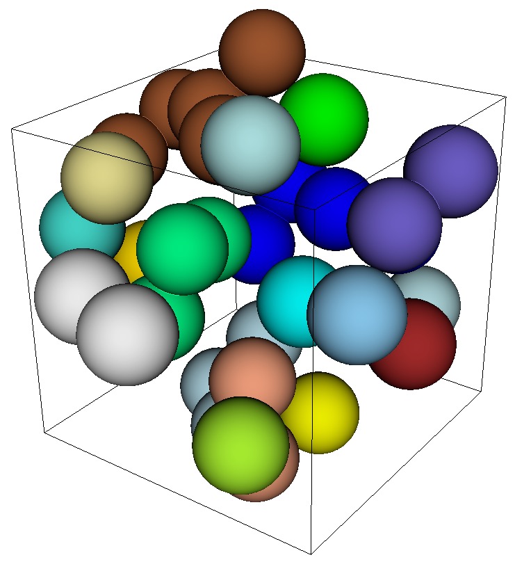
Figure 301: Resulting periodic mesh generated from example input.
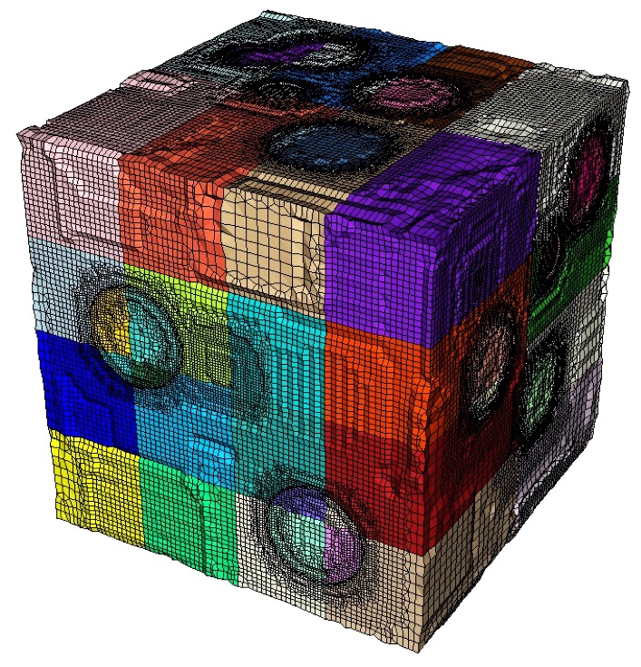
Figure 302: Six faces of the RVE from above example illustrating periodicity on a 32 processor decomposition. Note that top three images are a mirror image of the bottom three images.
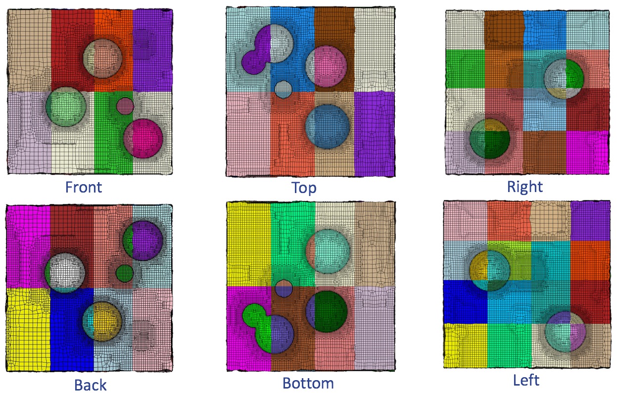
5.4.11.12.13 Check for periodic geometry
Command: check_periodic Check for periodic geometry |
Input file command: check_periodic <arg> |
Command line options: -cp <arg> |
Argument Type: on, off, only |
Input arguments: off (0) |
on (1) |
only (2) |
Command Description:
When using the periodic option with a Cartesian base grid, the input geometry must be periodic with respect to the grid bounding box in order to meet the minimum requirements of a valid periodic mesh. The bounding box must span exactly one period in each dimension. If this requirement is not met, a valid mesh may still be generated, however, periodicity will not be guaranteed. The check_periodic option is used to check this requirement. See also check_periodic_tol to set the tolerance for checking periodicity.
Options:
ON: The check_periodic option is ON by default to ensure periodicity is enforced. Sculpt will fail if the geometry and bounding box do not meet the requirements for periodicity.
OFF: Turning this option OFF will by-pass this check and attempt to generate the mesh even if periodic requirements are not met.
ONLY: The ONLY option will perform a check for periodic requirements and report diagnostics. An exodus file (or files) will be produced with the name "check_periodic.0.0.x.x". A stair-step mesh of the domain will be produced with an additional 2 blocks: 999 and 998. Block 999 shows master cells that are not matched. Block 998 shows paired ghost cells that should have the same volume fraction as those in block 999, but do not. Sculpt will immediately stop execution after producing the "check_periodic.0.0.x.x" mesh. Note that 2 additional layers on all sides of the Cartesian grid will be present in the mesh. These are used internally in Sculpt for parallel ghosting.
The check_periodic option is ignored if the periodic option is OFF or set to false.
5.4.11.12.14 Tolerance used for periodic check
Command: check_periodic_tol Tolerance for checking periodicity |
Input file command: check_periodic_tol <arg> |
Command line options: -cpt <arg> |
Argument Type: floating point value |
Command Description:
Used on conjunction with the check_periodic option. It specifies a tolerance value when checking periodicity. Check periodic option checks the difference between computed volume fractions for cells on the overlay grid that are separated by exactly one period. The periodic tolerance is the allowable volume fraction difference between cells separated by one period. Default value is 1e-6.
5.4.11.12.15 Periodic Mesh Axis
Command: periodic_axis Axis periodicity is about |
Input file command: periodic_axis <arg> |
Command line options: -pax <arg> |
Argument Type: six floating point values |
Command Description:
For an unstructured base grid, specifies an axis about which the nodes in the master (leading) nodesets will be rotated about to produce the slave (trailing) nodesets. Six floating point numbers are specified, the first three define the origin of the axis and the last three define the axis direction. This option must be used with –periodic (-per), –periodic_nodesets (-pns), and –input_mesh (-im) options. If the –periodic (-per) option is used without the –periodic_axis option, the transformation between leading and trailing nodesets is assumed to be pure translation.
5.4.11.12.16 Periodic Nodeset Ids
Command: periodic_nodesets Nodesets ids of master/slave nodesets |
Input file command: periodic_nodesets <arg> |
Command line options: -pns <arg> |
Argument Type: integer(s) >= 0 |
Command Description:
For an unstructured base grid, specifies the master-slave (leading-trailing) nodeset pairs. Master nodesets should be able to be translated or rotated about a specified axis to produce the nodes in the slave nodesets. Nodesets must be specified in pairs, where each master (leading) nodeset corresponds to a single slave (trailing) nodeset. Each nodeset pair must maintain an identical translation or rotation. If a rotation is used, the axis and origin of rotation must be specified with the –periodic_axis (-pax) option. This option should be used with –periodic (-per), –periodic_nodesets (-pns), and –input_mesh (-im) options.)
Figure 303: Unstructured input mesh used to generate periodic mesh. Matching leading and trailing nodesets are defined in the exodus file.
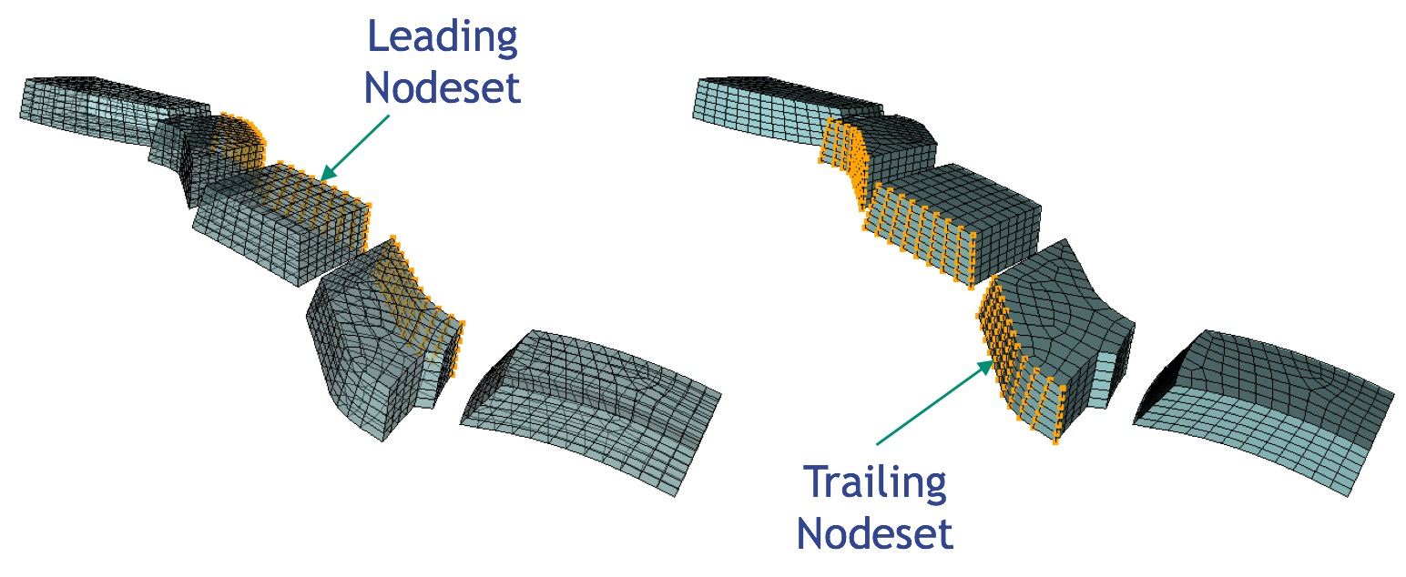
5.4.11.12.17 Write the ghost layers for debug
Command: build_ghosts Write ghost layers to exodus files for debug |
Input file command: build_ghosts |
Command line options: -bg |
Command Description:
If set, this option will dump the ghost hexes at the boundaries of processor domains to the exodus files. This is used only for debugging.
5.4.11.12.18 Volume Fraction Calculation Method
Command: vfrac_method Set method for computing volume fractions |
Input file command: vfrac_method <arg> |
Command line options: -vm <arg> |
Argument Type: integer (1, 2) |
Input arguments: cth (0) |
cth (1) |
r3d (2) |
Command Description:
Sets the method used for computing volume fractions from geometry input. Two options are currently available:
CTH (1): The default method. It uses the CTH third party library from Sandia Laboratories for approximating intersections using an adaptive ray firing method to determine inside-outside status of multiple locations within a grid cell. This method can be used with STL and all valid primitive types defined by the diatom format.
R3D (2): Uses the R3D third party library developed by Los Alamos Laboratories. Machine precision intersection calculations are performed to generate accurate volume fractions from the STL description. This method is valid for STL and diatom input packages specifying STL input files. Non STL format geometry defined in the diatom file will be ignored for this format.
5.4.11.13 Sculpt Overlay Grid Specification
Sculpt options for setting up the overlay grid. Sculpt is an overlay-grid method that requires a base mesh that it will modify to generate the final mesh. The base mesh can be in the form of a Cartesian grid, but can also be any general unstructured hexahedral mesh defined in an exodus file (see the input_mesh option). Pamgen can also be used to generate an unstructured base mesh (see input_mesh_pamgen).
When an overlay Cartesian grid is used as the basis for the all-hex mesh that will be produced, the bounds and size of the cells defining the grid must be specified. The Cartesian grid can be defined in one of two ways:
Define the bounding box and number of intervals in each coordinate direction. (xmin, ymin, zmin, xmax, ymax, zmax, nelx, nely, nelz)
Define a cell_size. Sculpt will then automatically define the Cartesian grid coordinates and intervals by evaluating the bounding box of the input geometry and adding a small number of cells in each coordinate direction.
Overlay Grid Specification --overlay -ovr |
--nelx -x <arg> Num cells in X in overlay Cartesian grid |
--nely -y <arg> Num cells in Y in overlay Cartesian grid |
--nelz -z <arg> Num cells in Z in overlay Cartesian grid |
--xmin -t <arg> Min X coord of overlay Cartesian grid |
--ymin -u <arg> Min Y coord of overlay Cartesian grid |
--zmin -v <arg> Min Z coord of overlay Cartesian grid |
--xmax -q <arg> Max X coord of overlay Cartesian grid |
--ymax -r <arg> Max Y coord of overlay Cartesian grid |
--zmax -s <arg> Max Z coord of overlay Cartesian grid |
--cell_size -cs <arg> Cell size (nelx, nely, nelz ignored) |
--align -a Automatically align geometry to grid |
--bbox_expand -be <arg> Expand tight bbox by percent |
--input_mesh -im <arg> Input Base Exodus mesh |
--input_mesh_blocks -imb <arg> Block ids of Input Base Exodus mesh |
--input_mesh_material -imm <arg> Material definition with input mesh |
--input_mesh_pamgen -imp <arg> Input Base mesh defined by Pamgen |
5.4.11.13.1 Number of Intervals X
Command: nelx Num cells in X in overlay Cartesian grid |
Input file command: nelx <arg> |
Command line options: -x <arg> |
Argument Type: integer > 0 |
Command Description:
Defines the number of intervals in the x direction of the base Cartesian grid used for defining the volume fraction definition and meshing For best results the intervals specified should result in approximately equilateral cells.
See also nely, nelz
5.4.11.13.2 Number of Intervals Y
Command: nely Num cells in Y in overlay Cartesian grid |
Input file command: nely <arg> |
Command line options: -y <arg> |
Argument Type: integer > 0 |
Command Description:
Defines the number of intervals in the y direction of the base Cartesian grid used for defining the volume fraction definition and meshing For best results the intervals specified should result in approximately equilateral cells.
See also nelx, nelz
5.4.11.13.3 Number of Intervals Z
Command: nelz Num cells in Z in overlay Cartesian grid |
Input file command: nelz <arg> |
Command line options: -z <arg> |
Argument Type: integer > 0 |
Command Description:
Defines the number of intervals in the z direction of the base Cartesian grid used for defining the volume fraction definition and meshing For best results the intervals specified should result in approximately equilateral cells.
See also nelx, nely
5.4.11.13.4 Xmin Bounding Box Range
Command: xmin Min X coord of overlay Cartesian grid |
Input file command: xmin <arg> |
Command line options: -t <arg> |
Argument Type: floating point value |
Command Description:
Defines the minimum x coordinate of the bounding box or range of the Cartesian mesh to be used for meshing.
See also ymin, zmin, xmax, ymax, zmax.
5.4.11.13.5 Ymin Bounding Box Range
Command: ymin Min Y coord of overlay Cartesian grid |
Input file command: ymin <arg> |
Command line options: -u <arg> |
Argument Type: floating point value |
Command Description:
Defines the minimum y coordinate of the bounding box or range of the Cartesian mesh to be used for meshing.
See also xmin, zmin, xmax, ymax, zmax.
5.4.11.13.6 Zmin Bounding Box Range
Command: zmin Min Z coord of overlay Cartesian grid |
Input file command: zmin <arg> |
Command line options: -v <arg> |
Argument Type: floating point value |
Command Description:
Defines the minimum z coordinate of the bounding box or range of the Cartesian mesh to be used for meshing.
See also xmin, ymin, xmax, ymax, zmax.
5.4.11.13.7 Xmax Bounding Box Range
Command: xmax Max X coord of overlay Cartesian grid |
Input file command: xmax <arg> |
Command line options: -q <arg> |
Argument Type: floating point value |
Command Description:
Defines the maximum x coordinate of the bounding box or range of the Cartesian mesh to be used for meshing.
See also xmin, ymin, zmin, ymax, zmax.
5.4.11.13.8 Ymax Bounding Box Range
Command: ymax Max Y coord of overlay Cartesian grid |
Input file command: ymax <arg> |
Command line options: -r <arg> |
Argument Type: floating point value |
Command Description:
Defines the maximum y coordinate of the bounding box or range of the Cartesian mesh to be used for meshing.
See also xmin, ymin, zmin, xmax, zmax.
5.4.11.13.9 Zmax Bounding Box Range
Command: zmax Max Z coord of overlay Cartesian grid |
Input file command: zmax <arg> |
Command line options: -s <arg> |
Argument Type: floating point value |
Command Description:
Defines the maximum z coordinate of the bounding box or range of the Cartesian mesh to be used for meshing.
See also xmin, ymin, zmin, xmax, ymax.
5.4.11.13.10 Cell Size
Command: cell_size Cell size (nelx, nely, nelz ignored) |
Input file command: cell_size <arg> |
Command line options: -cs <arg> |
Argument Type: floating point value |
Command Description:
Defines a target edge size for the cells of the base Cartesian grid. Both interval and cell_size can not be specified simultaneously. If cell_size is used without a range specification, a bounding box of the geometry will be computed and used as the default range.
5.4.11.13.11 Align
Command: align Automatically align geometry to grid |
Input file command: align |
Command line options: -a |
Command Description:
The align option will attempt to orient the Cartesian grid with the main dimensions of the geometry. This is done by defining a tight bounding box around the geometry using an optimization procedure where the objective is to minimize the difference in volume between an enclosing box and the geometry. Using the align command will override any bounding box parameters previously entered and will build an "aligned" bounding box around the full geometry. It is currently only implemented for STL geometry and will ignore any other diatom definitions. Note that this option will also write temporary stl and diatom files to the working directory.
5.4.11.13.12 Bounding Box Expansion Factor
Command: bbox_expand Expand tight bbox by percent |
Input file command: bbox_expand <arg> |
Command line options: -be <arg> |
Argument Type: floating point value |
Command Description:
Sculpt will measure a tight bounding box of the input model and expand the box by the specified percentage in x, y and z. Input value can be any positive or negative floating point value where 1.0 represents 100 percent expansion. If not specified, the default will add about 2.5 cell widths to the bounding box on each side. This option should be used with the cell_size option. It will be ignored if a specific bounding box has been defined (ie. xmin, ymin, etc...).
5.4.11.13.13 Input Base Exodus Mesh
ommand: input_mesh Input Base Exodus mesh |
Input file command: input_mesh <arg> |
Command line options: -im <arg> |
Argument Type: file name with path |
Command Description:
Option to import an Exodus file to use as the base mesh for Sculpt. Sculpt’s meshing procedure requires a base mesh from which geometry is recovered and captured. The default base mesh is a Cartesian grid that is defined by specifying a bounding box and intervals. The input_mesh option permits a general hexahedral mesh to be used as the base mesh instead of a Cartesian grid. This option currently supports a serial and parallel Exodus files containing HEX8 elements with any number of blocks.
Figure 304: An exodus file is used as the base mesh for Sculpt and STL files describe the geometry to be sculpted.
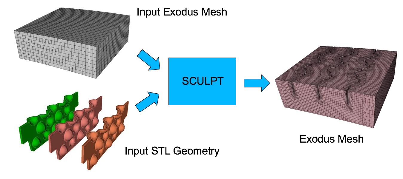
decomp -p 4 simple-mesh.g |
simple-mesh.g.4.0 |
simple-mesh.g.4.1 |
simple-mesh.g.4.2 |
simple-mesh.g.4.3 |
input_mesh = simple-mesh.g |
If the -j 4 option is used, sculpt will look for 4 meshes in the current working directory with the appropriate root and extension.
Four different options are supported for describing the geometry when using the input_mesh option:
stl_file: A single file containing a water-tight faceted description of the geometry. Note that only the portion of the STL file completely contained within the base mesh will be represented in the final mesh.
diatom_file: May contain analytic descriptions of geometric primitives and/or references to multiple STL files.
input_spn: The materials of the cells in the spn file are mapped onto the elements of the input mesh using inverse distance-weighted interpolation. As with the stl and diatom files, only the portion of the spn file completely contained within the base mesh will be represented in the final mesh. The input_mesh_blocks option can be used in conjunction with the spn_file option to limit the scope of the mapping of material from the spn file to the mesh file. If this options is used, only elements in the specified blocks will get mapped to. For more details, see the input_mesh_blocks option.
Element Variables: The geometry may also be described by element variables in the Exodus file. Element variables should represent material volume fractions where the sum of element variables for any one cell should be between 0.0 and 1.0. Any number of element variables may be used where each unique variable defined will describe an element block in the final Exodus mesh produced. if the sum of element variables is less than 1.0 for any one element, a void material will be assumed and removed from the base mesh unless the mesh_void option is used.
Limitations:
An STL file and element variables cannot be used in the same input. If element variables are present in the Exodus file and an STL or Diatom file is used, the element variables will be ignored.
If an input mesh is used, any Cartesian grid specifications will be ignored (ie. nelx, xmin, xmax).
The adapt_type option will work only for an exodus input mesh that defines a mapped mesh. Adapt types vfrac_average (4) and vfrac_difference (6) are currently the only criteria supported with the input_mesh option.
5.4.11.13.14 Blocks of Input Base Exodus Mesh
Command: input_mesh_blocks Block ids of Input Base Exodus mesh |
Input file command: input_mesh_blocks <arg> |
Command line options: -imb <arg> |
Argument Type: integers > 0 |
Command Description:
This option is valid when specifying both input_mesh and spn_file. Using this option, the materials of the cells in the spn file are mapped onto only the elements of the specified blocks in the input_mesh file. The remaining blocks are treated as void. The behavior without this option maps the materials of the cells in the spn file onto elements of all blocks in the input_mesh file.
5.4.11.13.15 Material Definition with Input Mesh
Command: input_mesh_material Material definition with input mesh |
Input file command: input_mesh_material <arg> |
Command line options: -imm <arg> |
Argument Type: integers > 0 |
Input arguments: geometry (0) |
blocks (1) |
proximity_blocks (2) |
Command Description:
This option is valid when specifying an ’input_mesh’ . Using this option, the material definition in the final mesh may be defined based on the material definitions on the geometry, or based on the block ids of the input mesh. For example, a diatom file defining geometry would have materials defined which are used to define the materials in the final mesh. The default is to use material definitions on the geometry. Possible options are:
geometry (0): Material defined by geometry. Block definitions in input file will be ignored. Instead, only the geometry defined from the STL or diatom geometry definition will be respected.
blocks (1): Material defined by blocks in input mesh. Both the geometry definition defined by the STL/diatom file and by the block definition in the input file will be used to construct the mesh. Block definitions used in the final mesh will be defined only by the input_mesh blocks, ignoring any material definitions in the diatom file. Note that pillowing may be required to maintain mesh quality where interior intersecting interfaces between STL/diatom geometry and block geometry occur. When used with the mesh_void option, element block groupings are made only for the interior of the STL/diatom geometry. Elements in the void region are assigned to the designated void_mat
- proximity_blocks (2): Material defined by blocks in input mesh based on proximity method. Geometric interfaces in the final mesh will be defined based on the STL/diatom definition, similar to the geometry (0) method. Material/block assignment for elements is defined only by the proximity of individual elements contained within the regions defined by blocks in the input mesh. Block assignment is made by collecting all elements in the final mesh whose centroid falls within a given block in the input mesh. Note that this method avoids the interior intersections and subsequent poor mesh quality that may result from the blocks (1) method described above. As a result, interior interfaces may be non-continuous (stair-step). In order to avoid collisions between the material ID defined in the diatom file and those defined in the input_mesh, block IDs in the final mesh are assigned based on the following definition:
ID = (diatom_material_ID-1)*max_input_mesh_block_ID + input_mesh_block_ID
If the max_input_mesh_block_ID is less than the max_diatom_material_ID, then the following definition is used:ID = (input_mesh_block_ID-1)*max_diatom_material_ID + diatom_material_ID
Figure 305: Example of the resulting meshes using the different options for input_mesh_material. In this case, geometry is defined by an STL file (sphere) and input_mesh is a brick containing 8 different material blocks.
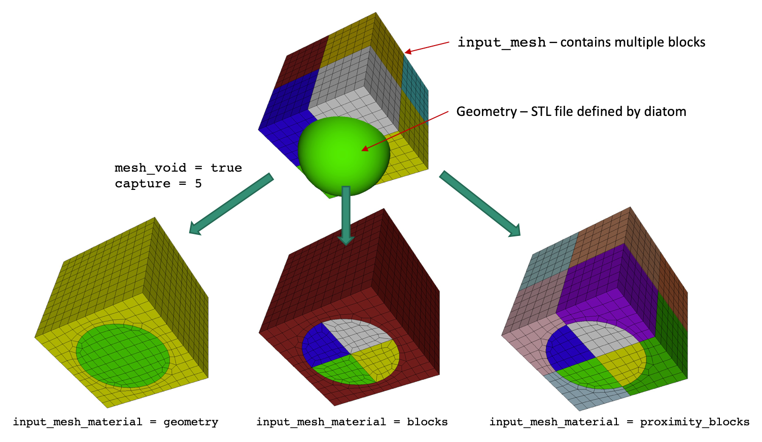
5.4.11.13.16 Input Base mesh defined by Pamgen
Command: input_mesh_pamgen Input Base mesh defined by Pamgen |
Input file command: input_mesh_pamgen <arg> |
Command line options: -imp <arg> |
Argument Type: file name with path |
Command Description:
Option to use Pamgen to create a base mesh for Sculpt. Pamgen is an open source meshing tool developed at Sandia for generating hexahedral meshes from geometric primitives. In addition to being a stand-alone meshing solution, it is a parallel tool that is integrated as an inline meshing tool for Sandia’s shock physics simulation tool, Alegra. Pamgen has also been integrated in Sculpt as a solution for automatically defining a base mesh.
mesh |
radial trisection |
trisection blocks, 2 |
zmin -0.00075 |
numz 1 |
zblock 1 1. interval 8 |
numr 3 |
rblock 1 2.0 interval 8 |
rblock 2 3.0 interval 8 |
rblock 3 4.0 interval 8 |
numa 1 |
ablock 1 90. interval 24 |
end |
set assign |
nodeset, ilo, 100 |
block sideset, ihi, 45, 2 |
end |
end |
For a full description of Pamgen and input parameters see the following document:
David M. Hensinger, Richard R. Drake, James G. Foucar, Thomas A. Gardiner, "Pamgen, a Library for Parallel Generation of Simple Finite Element Meshes", Sandia Report SAND2008-1933 (2008)
Figure 306: Base mesh generated by pamgen using the above input parameters. Colors represent 4 different processors when used in parallel mode.
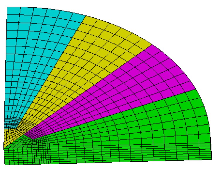
Similar to the input_mesh option, the same geometry input options are available. They include stl_file, diatom_file and input_spn. See the input_mesh option for additional details and limitations.
5.4.11.14 Sculpt Smoothing
Sculpt options for specifying how the mesh will be smoothed following mesh generation.
Sculpt includes a tiered approach to smoothing to improve element quality. It starts by applying smoothing to all nodes in the mesh and progressively restricts the smoothing operations to only those nodes that fall below a user-defined scaled Jacobian threshold. Default numbers of iterations and thresholds for each smoothing phase have been tuned for general use, however it may be worthwhile to adjust these parameters. The three smoothing phases include:
Laplacian Smoothing: Applied to all elements. Very inexpensive fast approach to improve quality, but can result in degraded element quality if applied to excess. A fixed default of 2 iterations is applied to all hexes. Increasing the num_laplace parameter can improve some cases, especially convex shapes.
Optimization Smoothing: Applied only to elements who’s scaled Jacobian falls below the opt_threshold parameter (default 0.6) and their surrounding elements. This approach uses a more expensive optimization technique to improve regions of elements simultaneously. The max_opt_iters parameter can control the maximum number of iterations applied (default is 5). Iterations will terminate, however, if no further improvement is detected. Because this method optimizes node locations simultaneously, neighboring nodes with competing optimum can sometimes limit mesh quality.
Spot Optimization: Also known as parallel coloring, is applied only to elements who’s element quality falls below the pcol_threshold parameter (default 0.2). This technique is the most expensive of the techniques, but focusses only on nodes that are immediately adjacent to poor quality hexes. Each node is smoothed independently of its neighbors, and may require a high number of iterations using the max_pcol_iters to achieve desired results. Increasing the pcol_threshold and max_pcol_iters may yield improved results.
Smoothing --smoothing -smo |
--smooth -S <arg> Smoothing method |
--csmooth -CS <arg> Curve smoothing method |
--laplacian_iters -LI <arg> Number of Laplacian smoothing iterations |
--max_opt_iters -OI <arg> Max. number of parallel Jacobi opt. iters. |
--opt_threshold -OT <arg> Stopping criteria for Jacobi opt. smoothing |
--curve_opt_thresh -COT <arg> Min metric at which curves won't be honored |
--max_pcol_iters -CI <arg> Max. number of parallel coloring smooth iters. |
--pcol_threshold -CT <arg> Stopping criteria for parallel color smooth |
--max_gq_iters -GQI <arg> Max. number of guaranteed quality smooth iters. |
--gq_threshold -GQT <arg> Guaranteed quality minimum SJ threshold |
--geo_smooth_max_deviation -GSM <arg> Geo Smoothing Maximum Deviation |
5.4.11.14.1 Smooth
Command: smooth Smoothing method |
|
Input file command: smooth <arg> |
Command line options: -S <arg> |
Argument Type: integer (0, 1, 2, 3) |
Input arguments: off (0) |
default (1) |
on (1) |
fixed_bbox (2) |
no_surface_projections (3) |
to_geometry (4) |
to_geom (4) |
geo_smooth (5) |
geometry_smoothing (5) |
geo_smoothing (5) |
Automatic adjustment of node locations following meshing to improve element quality. Controls the combined Laplacian and optimization smoothing procedures applied to volume and surface nodes (see csmooth for curve smoothing options) Uses the laplacian_iters, max_opt_iters, opt_threshold, max_pcol_iters, pcol_threshold, mqx_gq_iters and gq_threshold arguments to control the sensitivity and aggressiveness of the smoothing operations. In most cases, the default options for these parameters are sufficient, however increasing iterations or threshold values, while potentially causing longer run times, may result in improved mesh quality.
Smoothing will adjust the location of nodes on surfaces, projecting them to an approximated surface representation defined by interface reconstruction from volume fractions. In addition to turning smoothing on and off, the surface projection characteristics can be adjusted using the bbox_fixed and no_surface_projections options.
off (0): No volume and surface smoothing is performed.
on/default (1): (Default) Combined Laplacian/Optimization (Hybrid) smoothing both surface and volumes. Automatic boundary buffer layer improvement is performed at interior surfaces intersecting the domain boundary.
fixed_bbox (2): Uses standard hybrid smoothing procedure (option 1), however nodes at the the domain boundaries will be projected to one of the six planes of the bounding box or unstructured input_mesh. This option turns off the automatic boundary buffer improvement.
no_surface_projections (3): Uses the fixed_bbox method, however interior surfaces are not projected. This can result in smoother interior surface representations for microstructures models. This is effective in smoothing noisy surface data, but can potentially reduce overall volume. The laplacian_iters option will control the amount of smoothing that will occur, with higher numbers of iterations resulting in a smoother surface representation, but also resulting in more reduction in geometric volume. This method is default for microstructures file formats.
to_geometry (4): When used with the capture option, smoothing will also move nodes to the closest geometry entity. It must currently be used with capture to ensure that curves and surfaces are first identified and associated with boundary mesh entities. This option will only work with STL or diatom input that contains STL geometry.
geo_smooth (5): Similar to the smooth = to_geometry option, it is also intended to be used with the capture option. With the geo_smooth option, nodes are initially projected to the closest geometry entity. However, following the initial projection, Sculpt will utilize the Laplacian smoothing operation, similar to the smooth = no_surface_projections option, to effectively remove noise and local deviations in the geometry definition. The laplacian_iters option will control the amount of geometric smoothing that will occur. The optional command geo_smooth_max_deviation can also be used to control the maximum distance any individual node location can deviate from its original geometry definition.
Boundary Buffer Improvement: Sculpt’s smoothing procedures will use an automatic boundary buffer improvement method. It will attempt to improve the quality of hexes where interior surfaces are close to tangent with the bounding box. This can result in nodes that may not lie precisely on the planes of the domain boundary. The fixed_bbox (2) and no_surface_projections (3) options will turn off the automatic boundary buffer improvement.
5.4.11.14.2 Curve Smoothing
Command: csmooth Curve smoothing method |
|
Input file command: csmooth <arg> |
Command line options: -CS <arg> |
Argument Type: integer (0, 1, 2, ...6) |
Input arguments: off (0) |
circle (1) |
hermite (2) |
average_tangent (3) |
neighbor_surface_normal (4) |
vfrac (5) |
linear (6) |
off (0): No curve smoothing will be performed.
circle (1): Nodes projected to a fitted circle defined current node and its two neighbors.
hermite (2): Nodes projected based on Hermite interpolation. Note that this method can only be used in serial (-j 1)
average_tangent (3): Nodes projected based on average tangent of neighbors. Note that this method may not be parallel serial consistent.
neighbor_surface_normal (4): Nodes projected based on neighboring surface normals and the resulting intersecting planes.
vfrac (5): (Default) Nodes projected to initial curve interface defined from the original volume fraction data.
linear (6): Nodes projected to the linear segment defined by the node and its two immediate neighbors.
5.4.11.14.3 Laplacian Iterations
ommand: laplacian_iters Number of Laplacian smoothing iterations |
|
Input file command: laplacian_iters <arg> |
Command line options: -LI <arg> |
Argument Type: integer >= 0 |
Number of Laplacian smoothing iterations performed when Hybrid smoothing option is used. Default value is 2.
5.4.11.14.4 Maximum Optimization Iterations
Command: max_opt_iters Max. number of parallel Jacobi opt. iters. |
|
Input file command: max_opt_iters <arg> |
Command line options: -OI <arg> |
Argument Type: integer >= 0 |
Indicates the maximum number of iterations of optimization-based smoothing to perform. May complete sooner if no further improvement can be made. Default is 5
5.4.11.14.5 Optimization Threshold
Command: opt_threshold Stopping criteria for Jacobi opt. smoothing |
|
Input file command: opt_threshold <arg> |
Command line options: -OT <arg> |
Argument Type: floating point value (-1.0 -> 1.0) |
Indicates the value for scaled Jacobian where Optimization smoothing will be performed. Elements with scaled Jacobian less than opt_threshold and their neighbors will be smoothed. Default value is 0.6
5.4.11.14.6 Curve Optimization Threshold
Command: curve_opt_thresh Min metric at which curves won't be honored |
|
Input file command: curve_opt_thresh <arg> |
Command line options: -COT <arg> |
Argument Type: floating point value (-1.0 -> 1.0) |
Indicates the value for scaled Jacobian where if a node that falls on a curve has neighboring quads less than this value, then the smoothing will no longer honor the curve definition. Instead the optimization smoother will attempt to place the node to optimize the neighboring mesh quality, without regard for its placement on its owning curve.
Normally this value should be set close to zero to avoid too many nodes from floating off of their owning curves, however, if mesh quality is constrained by curve geometry, setting this value higher can help to avoid bad or poor quality elements. Default for this value is 0.1.
5.4.11.14.7 Maximum Parallel Coloring Iterations
Command: max_pcol_iters Max. number of parallel coloring smooth iters. |
|
Input file command: max_pcol_iters <arg> |
Command line options: -CI <arg> |
Argument Type: integer >= 0 |
5.4.11.14.8 Parallel Coloring Threshold
Command: pcol_threshold Stopping criteria for parallel color smooth |
|
Input file command: pcol_threshold <arg> |
Command line options: -CT <arg> |
Argument Type: floating point value (-1.0 -> 1.0) |
Indicates scaled Jacobian threshold for spot smoothing (also known as parallel coloring). A parallel coloring algorithm is used to uniquely identify and isolate nodes to be improved using optimization. Default is 0.2.
5.4.11.14.9 Maximum Guaranteed Quality Iterations
Command: max_gq_iters Max. number of guaranteed quality smooth iters. |
|
Input file command: max_gq_iters <arg> |
Command line options: -GQI <arg> |
Argument Type: integer >= 0 |
laplacian_iters = 0 |
max_opt_iters = 0 |
max_pcol_iters = 0 |
max_gq_iters = 100 |
5.4.11.14.10 Guaranteed Quality Threshold
Command: gq_threshold Guaranteed quality minimum SJ threshold |
|
Input file command: gq_threshold <arg> |
Command line options: -GQT <arg> |
Argument Type: floating point value (-1.0 -> 1.0) |
Indicates scaled Jacobian threshold for guaranteed quality smoothing. Default is 0.2. see also max_gq_iters
5.4.11.14.11 Geo Smooth Max Deviation
Command: geo_smooth_max_deviation Geo Smoothing Maximum Deviation |
|
Input file command: geo_smooth_max_deviation <arg> |
Command line options: -GSM <arg> |
Argument Type: floating point value (>= 0.0 |
Command Description: Used only in conjunction with the smooth = geo_smooth option. It controls the maximum distance any individual node can deviate from the geometry definition. If a smoothing operation computes a location that will move a node further than the prescribed geo_smooth_max_deviation value from the geometry, the node movement will be artificially limited by this value. If not specificied, no limitations will be placed on node movement due to smoothing operations when the smooth = geo_smooth is used. A value of zero (0) will constrain all nodes at interfaces to lie on the geometry, similar to the smooth = to_geometry option. When using this option, the maximum deviation from the geometry for any individual node will be reported in the MESH SUMMARY in the Sculpt ouput.
5.4.11.15 Sculpt Technical Description
This document provides a brief technical overview of the Sculpt application, a separate companion application to Cubit designed to generate all-hex meshes of complex geometries. Details on command arguments to Sculpt may be found here. Also information for using Cubit to set up input for Sculpt may be found here.
The method for generating an all-hex mesh employed by Sculpt is often referred to in the literature as an overlay-grid or mesh-first method. This differs significantly from the algorithms employed by Sweeping and Mapping, which are classified as geometry-first methods. Mapping and Sweeping start with the geometry, carefully fitting logical groupings of hexes to conform to a recognized topology. In contrast, the Sculpt method begins with a base Cartesian grid encompassing the geometry which is used as the basis for the mesh. Geometric features are carved or sculpted from the Cartesian grid and boundaries smoothed to create the final hex mesh. The obvious benefit of the Sculpt (mesh-first) method over Mapping and Sweeping (geometry-first) methods is there is no need to decompose the geometry into mappable or sweebable components, a process that can often be very time consuming, tedious and sometimes impossible. Input to Sculpt can be any geometry regardless of features and complexity.
The basic Sculpt procedure is illustrated in figure 1. Beginning with a Cartesian grid as the base mesh, shown in figure 1(a), a geometric description is imposed. Nodes from the base grid that are near the boundaries are projected to the geometry, locally distorting the nearby hex cells (figure 1(b)). A pillow layer of hexes is then inserted at the surfaces by duplicating the interface nodes on either side of the boundaries and inserting hexes (figures 1(c) and (d)). While constraining node locations to remain on the interfaces, smoothing procedures can now be employed to improve mesh quality of nearby hexes (figure 1(e)).
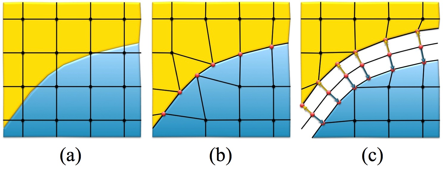
Figure 307: The procedure for generating a hex mesh using the Sculpt overlay grid method
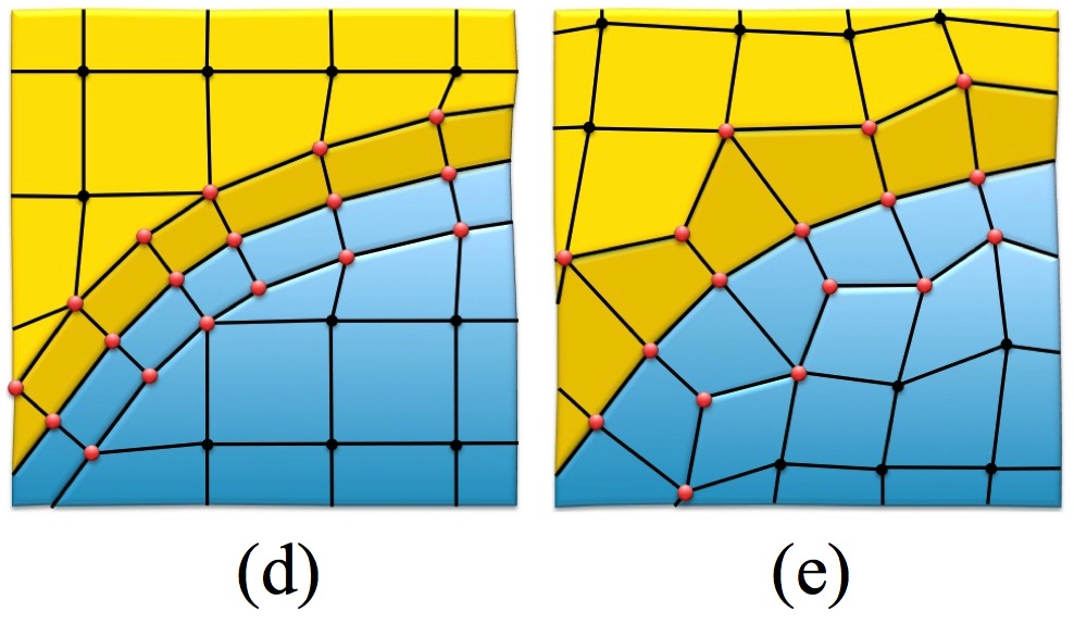
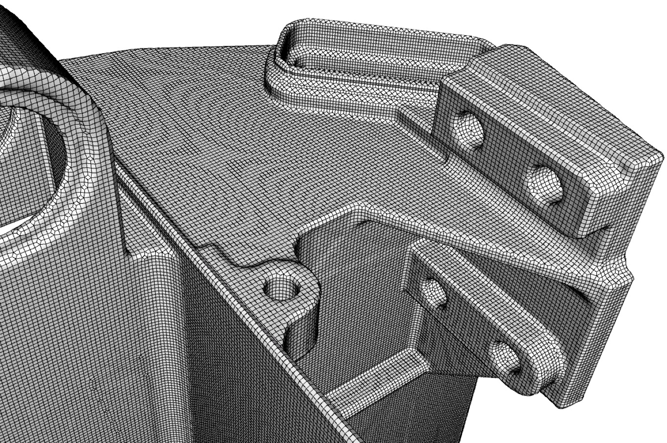
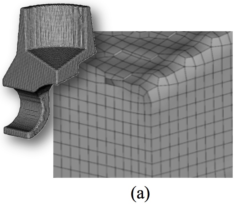
Figure 309: Examples of the same model meshed at two different resolutions showing a cutaway view of the mesh.
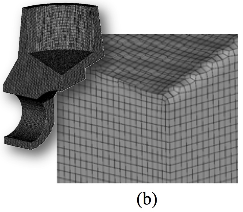
Figure 310: A representation of the procedure used to generate a hex mesh with Sculpt using Volume Fractions.
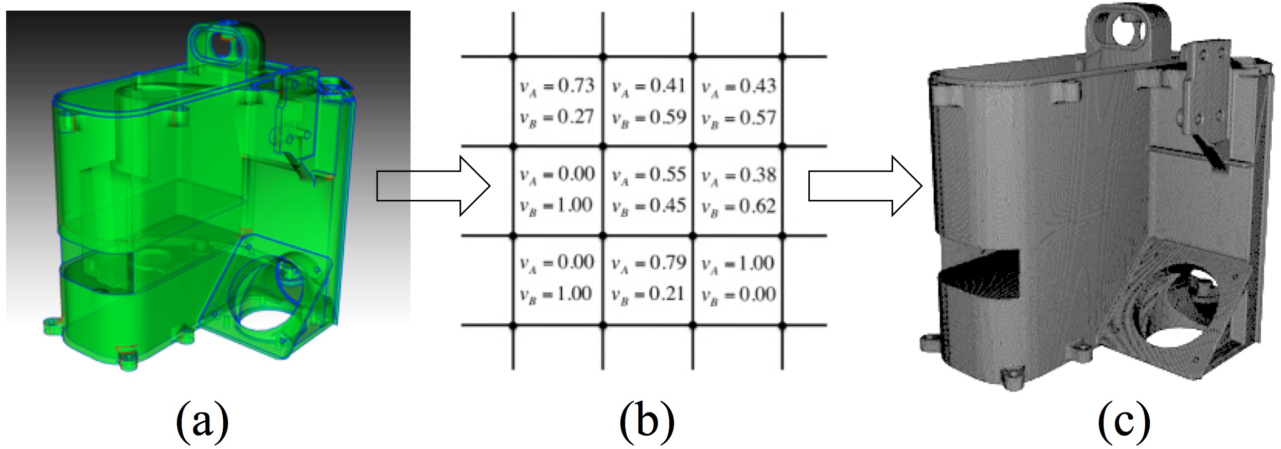
While acknowledging some loss in model fidelity in this new volume-fraction based geometric model, the advantage and time-savings to the analyst of being able to ignore troublesome geometry issues is enormous. At the same time it may be important to understand what the additional discrete approximations will make to solution accuracy and employ relevant engineering judgement in the use of this technology.
5.4.11.15.1 References
The following technical papers, written by the author of Sculpt, describe the Sculpt procedure in more depth. These papers were presented at the International Meshing Roundtable and are external links to pdf documents.
https://imr.sandia.gov/papers/imr20/Owen.pdf Describes the basic algorithms and mathematics used in the Sculpt procedure.
https://imr.sandia.gov/papers/imr21/RNOwen.pdf A brief description of the smoothing procedures used in Sculpt.
https://imr.sandia.gov/papers/imr22/IMR22_3_Owen.pdf Describes a study where computational results from Sculpt meshes are compared with Sweep meshes using the Sierra Solid Mechanics Tool as a comparison.
https://imr.sandia.gov/papers/imr24/03_IMR24_Owen.pdf Describes the refinement procedures used for generating adapted Sculpt meshes.
5.4.11.16 Sculpt Mesh Transformation
Mesh Transformation --transform -tfm |
--xtranslate -xtr <arg> Translate final mesh coordinates in X |
--ytranslate -ytr <arg> Translate final mesh coordinates in Y |
--ztranslate -ztr <arg> Translate final mesh coordinates in Z |
--scale -scl <arg> Scale final mesh coordinates by constant |
5.4.11.16.1 Translate Mesh Coordinates in X
Command: xtranslate Translate final mesh coordinates in X |
|
Input file command: xtranslate <arg> |
Command line options: -xtr <arg> |
Argument Type: floating point value |
5.4.11.16.2 Translate Mesh Coordinates in Y
Command: ytranslate Translate final mesh coordinates in Y |
|
Input file command: ytranslate <arg> |
Command line options: -ytr <arg> |
Argument Type: floating point value |
5.4.11.16.3 Translate Mesh Coordinates in Z
Command: ztranslate Translate final mesh coordinates in Z |
|
Input file command: ztranslate <arg> |
Command line options: -ztr <arg> |
Argument Type: floating point value |
5.4.11.16.4 Scale Mesh Coordinates by Constant
Command: scale Scale final mesh coordinates by constant |
|
Input file command: scale <arg> |
Command line options: -scl <arg> |
Argument Type: floating point value |
5.4.11.17 brick1.stl
solid Body 1 |
facet normal 0.000000e+00 0.000000e+00 1.000000e+00 |
outer loop |
vertex 5.000000e+00 5.000000e+00 5.000000e+00 |
vertex -5.000000e+00 5.000000e+00 5.000000e+00 |
vertex 5.000000e+00 -5.000000e+00 5.000000e+00 |
endloop |
endfacet |
facet normal 0.000000e+00 0.000000e+00 1.000000e+00 |
outer loop |
vertex 5.000000e+00 -5.000000e+00 5.000000e+00 |
vertex -5.000000e+00 5.000000e+00 5.000000e+00 |
vertex -5.000000e+00 -5.000000e+00 5.000000e+00 |
endloop |
endfacet |
facet normal 0.000000e+00 0.000000e+00 -1.000000e+00 |
outer loop |
vertex 5.000000e+00 -5.000000e+00 -5.000000e+00 |
vertex -5.000000e+00 -5.000000e+00 -5.000000e+00 |
vertex 5.000000e+00 5.000000e+00 -5.000000e+00 |
endloop |
endfacet |
facet normal -0.000000e+00 0.000000e+00 -1.000000e+00 |
outer loop |
vertex 5.000000e+00 5.000000e+00 -5.000000e+00 |
vertex -5.000000e+00 -5.000000e+00 -5.000000e+00 |
vertex -5.000000e+00 5.000000e+00 -5.000000e+00 |
endloop |
endfacet |
facet normal 0.000000e+00 -1.000000e+00 0.000000e+00 |
outer loop |
vertex -5.000000e+00 -5.000000e+00 5.000000e+00 |
vertex -5.000000e+00 -5.000000e+00 -5.000000e+00 |
vertex 5.000000e+00 -5.000000e+00 5.000000e+00 |
endloop |
endfacet |
facet normal 0.000000e+00 -1.000000e+00 -0.000000e+00 |
outer loop |
vertex 5.000000e+00 -5.000000e+00 5.000000e+00 |
vertex -5.000000e+00 -5.000000e+00 -5.000000e+00 |
vertex 5.000000e+00 -5.000000e+00 -5.000000e+00 |
endloop |
endfacet |
facet normal -1.000000e+00 -0.000000e+00 -0.000000e+00 |
outer loop |
vertex -5.000000e+00 5.000000e+00 5.000000e+00 |
vertex -5.000000e+00 5.000000e+00 -5.000000e+00 |
vertex -5.000000e+00 -5.000000e+00 5.000000e+00 |
endloop |
endfacet |
facet normal -1.000000e+00 -0.000000e+00 -0.000000e+00 |
outer loop |
vertex -5.000000e+00 -5.000000e+00 5.000000e+00 |
vertex -5.000000e+00 5.000000e+00 -5.000000e+00 |
vertex -5.000000e+00 -5.000000e+00 -5.000000e+00 |
endloop |
endfacet |
facet normal 0.000000e+00 1.000000e+00 0.000000e+00 |
outer loop |
vertex 5.000000e+00 5.000000e+00 5.000000e+00 |
vertex 5.000000e+00 5.000000e+00 -5.000000e+00 |
vertex -5.000000e+00 5.000000e+00 5.000000e+00 |
endloop |
endfacet |
facet normal 0.000000e+00 1.000000e+00 0.000000e+00 |
outer loop |
vertex -5.000000e+00 5.000000e+00 5.000000e+00 |
vertex 5.000000e+00 5.000000e+00 -5.000000e+00 |
vertex -5.000000e+00 5.000000e+00 -5.000000e+00 |
endloop |
endfacet |
facet normal 1.000000e+00 -0.000000e+00 0.000000e+00 |
outer loop |
vertex 5.000000e+00 -5.000000e+00 5.000000e+00 |
vertex 5.000000e+00 -5.000000e+00 -5.000000e+00 |
vertex 5.000000e+00 5.000000e+00 5.000000e+00 |
endloop |
endfacet |
facet normal 1.000000e+00 -0.000000e+00 0.000000e+00 |
outer loop |
vertex 5.000000e+00 5.000000e+00 5.000000e+00 |
vertex 5.000000e+00 -5.000000e+00 -5.000000e+00 |
vertex 5.000000e+00 5.000000e+00 -5.000000e+00 |
endloop |
endfacet |
endsolid Body 1 |
5.4.11.18 brick2.stl
solid Body 1 |
facet normal 0.000000e+00 0.000000e+00 1.000000e+00 |
outer loop |
vertex 1.500000e+01 5.000000e+00 5.000000e+00 |
vertex 5.000000e+00 5.000000e+00 5.000000e+00 |
vertex 1.500000e+01 -5.000000e+00 5.000000e+00 |
endloop |
endfacet |
facet normal 0.000000e+00 0.000000e+00 1.000000e+00 |
outer loop |
vertex 1.500000e+01 -5.000000e+00 5.000000e+00 |
vertex 5.000000e+00 5.000000e+00 5.000000e+00 |
vertex 5.000000e+00 -5.000000e+00 5.000000e+00 |
endloop |
endfacet |
facet normal 0.000000e+00 0.000000e+00 -1.000000e+00 |
outer loop |
vertex 1.500000e+01 -5.000000e+00 -5.000000e+00 |
vertex 5.000000e+00 -5.000000e+00 -5.000000e+00 |
vertex 1.500000e+01 5.000000e+00 -5.000000e+00 |
endloop |
endfacet |
facet normal -0.000000e+00 0.000000e+00 -1.000000e+00 |
outer loop |
vertex 1.500000e+01 5.000000e+00 -5.000000e+00 |
vertex 5.000000e+00 -5.000000e+00 -5.000000e+00 |
vertex 5.000000e+00 5.000000e+00 -5.000000e+00 |
endloop |
endfacet |
facet normal 0.000000e+00 -1.000000e+00 0.000000e+00 |
outer loop |
vertex 5.000000e+00 -5.000000e+00 5.000000e+00 |
vertex 5.000000e+00 -5.000000e+00 -5.000000e+00 |
vertex 1.500000e+01 -5.000000e+00 5.000000e+00 |
endloop |
endfacet |
facet normal 0.000000e+00 -1.000000e+00 -0.000000e+00 |
outer loop |
vertex 1.500000e+01 -5.000000e+00 5.000000e+00 |
vertex 5.000000e+00 -5.000000e+00 -5.000000e+00 |
vertex 1.500000e+01 -5.000000e+00 -5.000000e+00 |
endloop |
endfacet |
facet normal -1.000000e+00 -0.000000e+00 -0.000000e+00 |
outer loop |
vertex 5.000000e+00 5.000000e+00 5.000000e+00 |
vertex 5.000000e+00 5.000000e+00 -5.000000e+00 |
vertex 5.000000e+00 -5.000000e+00 5.000000e+00 |
endloop |
endfacet |
facet normal -1.000000e+00 -0.000000e+00 -0.000000e+00 |
outer loop |
vertex 5.000000e+00 -5.000000e+00 5.000000e+00 |
vertex 5.000000e+00 5.000000e+00 -5.000000e+00 |
vertex 5.000000e+00 -5.000000e+00 -5.000000e+00 |
endloop |
endfacet |
facet normal 0.000000e+00 1.000000e+00 0.000000e+00 |
outer loop |
vertex 1.500000e+01 5.000000e+00 5.000000e+00 |
vertex 1.500000e+01 5.000000e+00 -5.000000e+00 |
vertex 5.000000e+00 5.000000e+00 5.000000e+00 |
endloop |
endfacet |
facet normal 0.000000e+00 1.000000e+00 0.000000e+00 |
outer loop |
vertex 5.000000e+00 5.000000e+00 5.000000e+00 |
vertex 1.500000e+01 5.000000e+00 -5.000000e+00 |
vertex 5.000000e+00 5.000000e+00 -5.000000e+00 |
endloop |
endfacet |
facet normal 1.000000e+00 -0.000000e+00 0.000000e+00 |
outer loop |
vertex 1.500000e+01 -5.000000e+00 5.000000e+00 |
vertex 1.500000e+01 -5.000000e+00 -5.000000e+00 |
vertex 1.500000e+01 5.000000e+00 5.000000e+00 |
endloop |
endfacet |
facet normal 1.000000e+00 -0.000000e+00 0.000000e+00 |
outer loop |
vertex 1.500000e+01 5.000000e+00 5.000000e+00 |
vertex 1.500000e+01 -5.000000e+00 -5.000000e+00 |
vertex 1.500000e+01 5.000000e+00 -5.000000e+00 |
endloop |
endfacet |
endsolid Body 1 |
5.4.11.19 bricks.diatom
diatoms |
package 'Brick1' |
material 1 |
iterations 3 |
insert stl |
FILE = 'brick1.stl' |
endinsert |
endp |
package 'Brick2' |
material 2 |
iterations 3 |
insert stl |
FILE = 'brick2.stl' |
endinsert |
endp |
enddia |
5.4.12 Traditional
5.4.12.1 Bias, Dualbias
Applies to: Curves
Summary: Meshes a curve with node spacing biased toward one or both curve ends.
To use the bias scheme
On the Command Panel, click on Mesh and then Curve.
Click on the Mesh action button.
Enter the values for Select Curves. This can also be done using the Pick Widget function.
Select Bias from the drop-down menu.
Select the desired option from the drop-down menu and enter in the appropriate settings.
Click on Apply Size and then Mesh.
Curve <range> Scheme Bias
Curve <range> Scheme Bias {Factor|First_Delta|Fraction} <double> [Start Vertex <range>] [preview]
Curve <range> Scheme Dualbias {Factor|First_Delta|Fraction} <double> [preview]
Curve <range> Scheme Bias Fine Size <double>
{Coarse Size <double> | Factor <double>} [Start Vertex <range>] [preview]
Curve <range> Scheme Dualbias Fine Size <double>
{Coarse Size <double> | Factor <double>} [preview]
Curve <range> Scheme Multi_bias Start <size> [Fraction <value> <size>]... End <size> [Start Vertex <id>][Respect_intervals][preview]
Curve <range> Reverse Bias
Set Maximum Interval <int>
See also Surface Sizing Function Type Bias
See also Curve Scheme Stretch
The main differences between scheme bias and stretch are the following: scheme stretch does not use strict geometric series for node placement. If you specify scheme bias or dualbias using the "fine size" form, the interval count will be hard-set to a value that fills in the curve.
Auto Bias When using the command ’curve <range> scheme bias’ with no additional parameters, an ’auto’ setting will be enabled by default for tet and tri meshing. This scheme honors sizes set at a curve’s vertices and that vertex size will be used to create a biased edge mesh. For example, two volumes with different sizes set on the volumes are merged. The sizes at the vertices (averaged from sizes on the parent entities) will be used to create the biased edge mesh.
vertex <id> size <size>
Discussion: The Bias and DualBias schemes space the curve mesh unequally, placing more nodes towards (or away from) the ends of the curve according to a geometric progression. The ratio of successive edges is the "factor," which may be greater than or less than one. For bias, the series starts at the first vertex of the curve, or the "start vertex" if specified. For dualbias, the series starts at both ends of the curve and meets in the middle.
The command behaves differently depending on which set of parameters are specified. There are three basic variables: the interval count, the bias factor, or the first edge size. The curve length is a given, fixed quantity. The user can specify any two of these variables, and the third will be automatically determined.
If the "{Factor|First_Delta|Fraction}" form is specified, then the interval count is taken as a given. The interval count is whatever was specified previously by an interval count or size command (see Interval Assignment). If "Factor" is specified, then the first edge size will be automatically chosen so that the geometric progression of edges "fit" onto the curve. If "first_delta" is specified, then the first edge length is exactly that absolute value, and the "factor" is automatically chosen. If "fraction" is specified, then the first edge length is the curve length times that fraction, and again the "factor" is automatically chosen.
If the "fine size" is specified, then the first edge length is exactly that absolute value. If the "factor" is specified, then the interval count is automatically chosen. If an approximate coarse size is specified, then this also determines the factor, and again the interval count is automatically chosen. If a surface sizing function type bias is used, then the curves of the surface are sized using similar formulas.
If no start or end vertex is specified, the curve’s start vertex is used as the starting point of the bias. (A curve’s start vertex can be identified by listing the curve from the "Cubit>" prompt.) If a curve needs to have its nodes distributed towards the opposite end, it can be easily edited using the reverse bias command. Reversing the curve bias using this command is equivalent to setting a bias factor equal to the inverse of the original bias factor. Reversing the bias can be performed on both meshed and unmeshed curves. The maximum interval setting allows the user to set a maximum number of intervals on any bias curve. This value is doubled for a curve with a dualbias scheme. It can be easy to accidentally specify a very large number of intervals and this setting allows the user to place an upper limit the number of intervals.
The preview option will allow the user to preview mesh size and distribution on the curve before meshing.
The following figure shows the result of meshing edges with equal, bias and dualbias schemes.
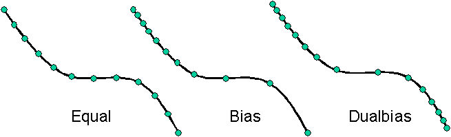
Multi Bias The multi-bias scheme allows several biases to be created on a single curve by specifying desired sizes at multiple locations along the curve (see Figure 312 below). The "start" and "end" sizes must be specified, and any number of fraction-size pairs may be specified, where the fraction value is between 0 and 1. If "Start Vertex" is given, the specified vertex is considered to have the fraction value of 0, with the opposite vertex having the fraction value of 1. If "respect_intervals" is not specified, the scheme will choose an appropriate number of intervals for the curve based on the given sizes.
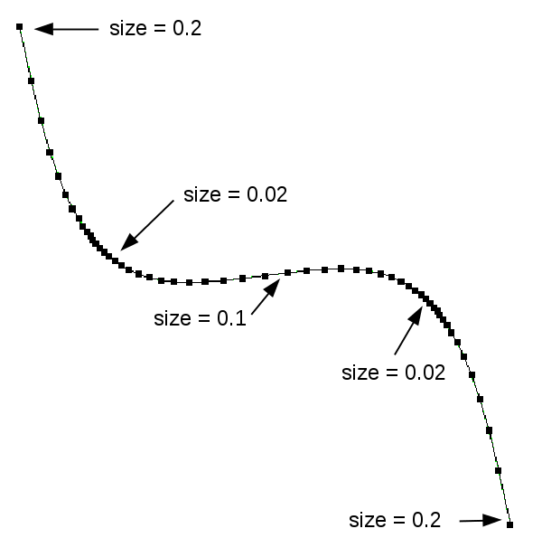
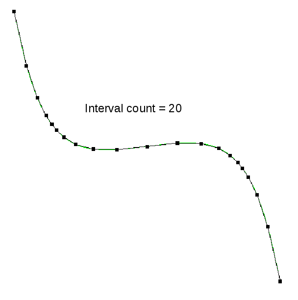
5.4.12.2 Circle
Applies to: Surfaces
Summary: Produces a circle-primitive mesh for a surface
Surface <range> Scheme [Sector] Circle [Interval <int>] [fraction <double>]
Discussion: The Circle scheme is used in regions that should be meshed as a circle. A "circle" consists of a single loop of bounding curves containing an even number of intervals. Thus, the circle scheme can be applied to circles, ellipses, ovals, and regions with "corners" (e.g. polygons). The bounding curves should enclose a convex region. Non-planar bounding loops can also be meshed using the circle primitive provided the surface curvature is not too great. The mesh resembles that obtained via polar coordinates except that the cells at the "center" are quadrilaterals, not triangles. See Figure 314 for an example of a circle mesh. Radial grading of the mesh may be achieved via the optional [intervals] input parameter. The Fraction option has the range 0 < fraction < 1 and defaults to 0.5. Fraction determines the size of the inner portion of the circle mesh relative to the total radius of the circle. The sector option was added to revert to legacy behavior which is not recommended.
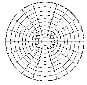
5.4.12.3 Curvature
Applies to: Curves
Summary: Meshes curves by adapting the interval size to the local curvature.
To mesh curves by adapting the interval size to the local curvature
On the Command Panel, click on Mesh and then Curve.
Click on the Mesh action button.
Enter the values for Select Curves. This can also be done using the Pick Widget function.
Select Curvature from the drop-down menu.
Enter the appropriate Value.
Click on Apply Size and then Mesh.
Curve <range> Scheme Curvature <double>
Discussion: The value of <double> controls the degree of adaptation. If zero, the resulting mesh will have nearly equal intervals. If greater than zero, the smallest intervals will correspond to the locations of largest curvature. If less than zero, the largest intervals will correspond to the locations of largest curvature. The default value of <double> is zero. Straight lines and circular arcs will produce meshes with near-equal intervals. The method for generating this mesh is iterative and may sometimes not converge. If the method does not converge, either the <double> is too large (over-adaptation) or the number of intervals is too small. Currently, the scheme does not work on periodic curves.
5.4.12.4 Equal
Applies to: Curves
Summary: Meshes a curve with equally-spaced nodes
To mesh an equally-spaced curve
On the Command Panel, click on Mesh and then Curve.
Click on the Mesh action button.
Enter the values for Select Curves. This can also be done using the Pick Widget function.
Select Equal from the drop-down menu.
Select Approximate Size, Auto Size or Interval.
Enter the appropriate settings.
Click on Apply Size and then Mesh.
Curve <range> Scheme Equal
See Interval Assignment for a description of how to set the number of nodes or the node spacing on a curve.
5.4.12.5 Hole
Applies to: Annular Surfaces
Summary: Useful on annular surfaces to produce a "polar coordinate" type mesh (with the singularity removed).
To create a polar coordinate-like mesh
On the Command Panel, click on Mesh and then Surface.
Click on the Mesh action button.
Enter the values for Select Surface. This can also be done using the Pick Widget function.
Select Hole from the drop-down menu.
Optionally, click on Advanced to further specify the settings.
Click on Apply Scheme and then Mesh.
Surface <surface_id_range> Scheme Hole [Rad_intervals <int>] [Bias <double>] [Pair Node <id> With Node <id>]
Discussion: A polar coordinate-like mesh with the singularity removed is produced with this scheme. The azimuthal coordinate lines will be of constant radius (unlike scheme map) The number of intervals in the azimuthal direction is controlled by setting the number of intervals on the inner and outer bounding loops of the surface (the number of intervals must be the same on each loop). The number of intervals in the radial direction is controlled by the user input, rad_intervals (default is one).
A bias may be put on the mesh in the radial direction via the input parameter bias. The default bias of 0 gives a uniform grading, a bias less than zero gives smaller radial intervals near the inner loop, and a bias greater than zero gives smaller radial intervals near the outer loop.
The correspondence between mesh nodes on the inner and outer boundaries is controlled with the pair node "<loop node-id> with node <loop node-id>" construct. One id on the inner loop and one id on the outer loop should be given to connect the two nodes by a radial mesh line. Not choosing this option may result in sub-optimal node pairings with possible negative Jacobians. To use this option, mesh the inner and outer curve loops and then determine the mesh node ids.
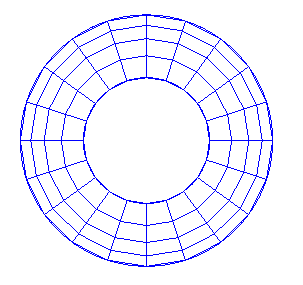
5.4.12.6 Mapping
Applies to: Surfaces, Volumes
Summary: Meshes a surface/volume with a structured mesh of quadrilaterals/hexahedra. To map on a surface
On the Command Panel, click on Mesh and then Surface.
Click on the Mesh action button.
Enter the values for Select Surface. This can also be done using the Pick Widget function.
Select Map from the drop-down menu.
Optionally, click on Advanced to further specify the settings.
Click on Apply Scheme and then Mesh.
To map on a volume
On the Command Panel, click on Mesh and then Volume.
Click on the Mesh action button.
Enter the values for Select Volumes. This can also be done using the Pick Widget function.
Select Map from the drop-down menu.
Click on Apply Scheme and then Mesh.
{Volume|Surface} <range> Scheme Map


Table 1. Listing of Logical Sides
Logical Side
Curve Groups
Side 1
Curve 1
Side 2
Curve 2
Side 3
Curve 3, Curve 4, Curve 5
Side 4
Curve 6


Set Mapping Constraint {ON|off}
Surface <range> Scheme Map [Direction {Options}]
If a projection direction is specified, the nodes are moved to the geometry in a straight line along the given direction. The direction can be specified using any of the direction options.
5.4.12.7 Pave
Applies to: Surfaces
Summary: Automatically meshes a surface with an unstructured quadrilateral mesh.
On the Command Panel, click on Mesh and then Surface.
Click on the Mesh action button.
Enter the values for Select Surface. This can also be done using the Pick Widget function.
Select Pave from the drop-down menu.
Select On, Off or Extend from the Paver Cleanup menu.
Click on Apply Scheme and then Mesh.
Surface <range> Scheme Pave Related Commands:
[Set] Paver Diagonal Scale <factor (Default = 0.9)> [set] Paver Grid Cell <factor (Default = 2.5)>[set] Paver LinearSizing {Off | ON} Mesh Adaptivity and Sizing Functions
[Set] Paver Smooth Method {DEFAULT | Smooth Scheme | Old}
[Set] Paver Cleanup {ON|Off|Extend}
Discussion: Paving (Blacker, 91; White, 97) allows the meshing of an arbitrary three-dimensional surface with quadrilateral elements. The paver supports interior holes, arbitrary boundaries, hard lines, and zero-width cracks. It also allows for easy transitions between dissimilar sizes of elements and element size variations based on sizing functions. Figure 318 shows the same surface meshed with mapping (left) and paving (right) schemes using the same discretization of the boundary curves.
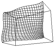
Figure 318: Map (left) and Paved (right) Surface Meshes
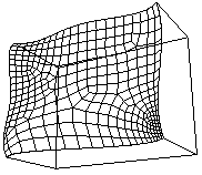
5.4.12.7.1 Element Shape Improvement
[set] Paver Smooth Method {DEFAULT | Smooth Scheme | Old}
5.4.12.7.2 Controlling Flattening of Elements
[set] Paver Diagonal Scale <factor (Default = 0.9)>
The range of for the scale factor is 0.5 to 1.0. A scale factor of 1.0 will force the element to be a parallelogram as long as it is on the mesh front. A value of 0.5 will allow the diagonal to be half its calculated length. The element may became triangular in shape with the two sides on the mesh front being collinear.
5.4.12.7.3 Controlling the Grid Search for Intersection Checking
[set] Paver Grid Cell <factor (Default = 2.5)>
The grid cell factor is a multiplier applied to the average element size, which then becomes the grid cell size. The surface’s bounding box is divided by this cell size to determine the number of cells in each direction. A larger cell size means each cell contains more nodes and edges. A smaller cell size means each cell has fewer nodes and edges. A larger cell size forces the intersection algorithm to check more potential intersections, which results in long paver times. A smaller cell size gives the intersection algorithm few edges to check (faster execution) but may result in missed intersections where the ratio of long to short element edges is great. Increase this value if the paver is missing intersections of elements.
5.4.12.7.4 Controlling the Paver Sizing Function
[set] Paver LinearSizing {Off | ON}
Setting paver linear sizing to "off" will keep the default behavior. The size of the element will be based on the side(s) of the element on the mesh front. For a discussion of sizing functions, including how to automatically set up size transitions, see Adaptive Meshing.
5.4.12.7.5 Controlling Paver Cleanup
[Set] Paver Cleanup {ON|Off|Extend}
The extend option attempts to group several defective nodes in a region that may be replaced with a template that has fewer defects. The images below show a mesh before and after using this option.
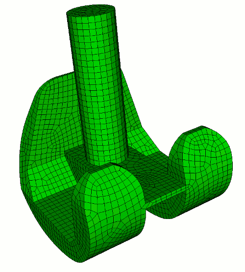
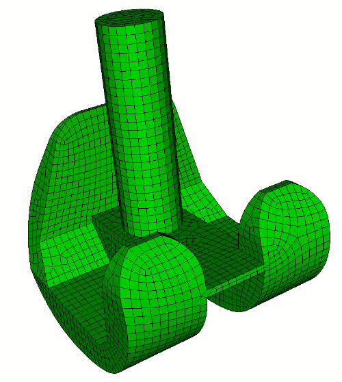
5.4.12.8 Pentagon
Applies to: Surfaces
Summary: Produces a pentagon-primitive mesh for a surface
Surface <range> Scheme Pentagon
Discussion: The pentagon scheme is a meshing primitive for 5-sided regions. It is similar to the triprimitive and polyhedron schemes, but is hard-coded for 5 sided surfaces.
5.4.12.9 Pinpoint
Applies to: Curves
Summary:Meshes a curve with node spacing specified by the user.
To pinpoint where to place nodes on a curve
On the Command Panel, click on Mesh and then Curve.
Click on the Mesh action button.
Enter the values for Select Curves. This can also be done using the Pick Widget function.
Select Pinpoint from the drop-down menu.
Enter the appropriate value for Distance(s) Along Curve:.
Click on Apply Size and then Mesh.
Curve <range> Scheme Pinpoint Location <list of doubles>
curve 2 scheme pinpoint location 1 4 5 6 6.2 6.4 6.6 9:
5.4.12.10 Polyhedron
Applies to: Surfaces and Volumes.
Summary: Produces an arbitrary-sided block primitive mesh for a surface or volume.
To use a polyhedron scheme on a volume or surface
On the Command Panel, click on Mesh.
Click on Volume or Surface.
Click on the Mesh action button.
Enter the values for Select Surfaces or Select Volumes. This can also be done using the Pick Widget function.
Select Polyhedron from the drop-down menu.
Click on Apply Scheme and then Mesh.
Volume <range> Scheme Polyhedron
Surface <range> Scheme Polyhedron
Discussion:
The polyhedron scheme is a meshing primitive for 2d and 3d n-sided regions. This is similar to the triprimitive , tetprimitive, and pentagon schemes, except rather than 3, 4, or 5 sides, it allows an arbitrary number of sides. The scheme works best on convex regions. Surfaces must have only one loop, and each vertex must be connected to exactly two curves on the surface (e.g., no hardlines). Volumes must have only one shell, each vertex must be connected to exactly three surfaces on the volume, and each surface should be meshed with scheme polyhedron. There are some interval assignment requirements as well, which should be automatically handled by Cubit.
If the polyhedron scheme is specified for the volume, then the surfaces of the volume are automatically assigned scheme polyhedron as well, unless they were hard-set by the user. Schemes should be specified on all volumes of an assembly prior to meshing any of them. Scheme polyhedron attaches extra data to volumes; if Cubit is behaving strangely, the user may need to explicitly remove that data with a reset volume all, or similar command.
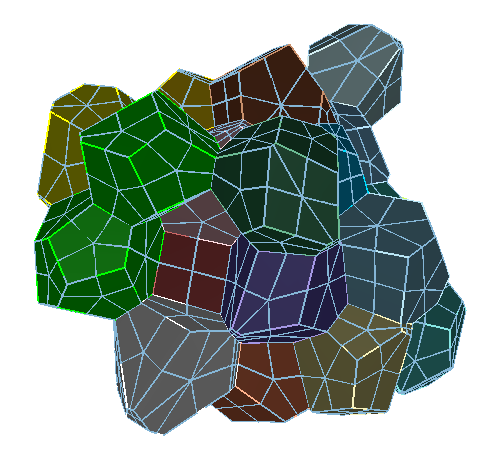
5.4.12.11 Quad Dominant
Applies to: Surfaces
Summary: Automatically meshes parametric surface geometry with quadrilaterals and triangles
To use a quad dominant scheme:
On the Command Panel, click on Mesh and then Surface.
Click on the Mesh action button.
Enter the appropriate value for Select Surfaces. This can also be done using the Pick Widget function.
Select QuadDominant from the drop-down menu.
Click Apply Scheme then click Mesh.
Surface <range> Scheme quad_dominant
After applying the quad_dominant surface scheme, set the volume meshing scheme to tetmesh and mesh. The volume will be filled with tetrahedral and wedge elements.
Figure 324:
Bracket meshed using the quad_dominant scheme. Triangles are colored in red.
5.4.12.12 Sphere
Applies to: Volumes topologically equivalent to a sphere and having one surface.
Summary: Generates a radially-graded hex mesh on a spherical volume.
Volume <range> Scheme Sphere [Graded_interval <int>] [Az_interval <int>] [Bias <val>] [Fraction <val>] [Max_smooth_iterations <int=2>]
Discussion: This scheme generates a radially-graded mesh on a spherical volume having a single bounding surface. The mesh is a straightforward generalization of the circle scheme for surfaces. The mesh consists of inner region and outer region. The inner region is a mesh of a cube and the outer region contains fronts that transition from cube surface to sphere surface. Parameters: The number of radial intervals in the outer region is controlled by the graded_interval input parameter. Azimuthal mesh lines in the outer portion of the sphere have constant radius. Azimuthal mesh lines in the outer portion of the sphere will have approximately constant radius. If graded_interval is not specified, a default number of intervals will be computed based on the interval size value assigned to the sphere volume.
The number of azimuthal intervals around the equator is controlled by the az_interval input parameter. To maintain symmetry, the az_interval will be rounded to the nearest multiple of 8. If az_interval is not specified, a default number of intervals will be computed based on the interval size value assigned to the sphere volume. The interval size will be used as the approximate size for elements on the inner mapped mesh. This normally results in interval sizes approximately 3X greater for elements at the sphere surface.
An alternative method for setting the az_interval on the sphere is to assign a specific number of intervals to the sphere volume. For example if volume 1 was a sphere, the comand volume 1 interval 40, if not otherwise defined, would set the value for az_interval to 40.
The bias parameter controls the amount of radial grading in the outer region of the mesh from the inner mapped mesh to the sphere surface. A bias = 1 will results in equal size intervals, while a bias < 1 will generate smaller intervals towards the sphere interior and a bias > 1 will generate smaller elements towards the sphere surface. If the bias parameter is not specified, a default bias will be computed so that element size gradually increases from the inner mapped mesh to the sphere surface. The default bias value will also be based on the interval size assigned to the sphere volume as it attempts to maintain approximately isotropic elements throughout the sphere.
The fraction parameter (between 0 and 1) determines what fraction of the sphere is occupied by the inner mapped mesh. The fraction is defined as ratio of the diagonal of the cube containing the mapped mesh to sphere’s diameter. The default value for fraction is 0.5. Interval sizes in the inner mapped mesh are normally constrained by the az_intervals. If az_intervals are not specified, element sizes in this region will be based upon the interval size assigned to the sphere volume.
The max_smooth_iterations parameter determines the number of smoothing iterations following initial definition of the sphere mesh. By default, the number of smoothing interations is set to 0, which will result in a symmetric mesh. Note that smoothing can improve the quality of the mesh, however, it may disturb the bias and fraction. When bias and fraction are critical then smoothing iterations should be set to 0.
Figure 325:
SPHERE MESH: fraction 0.3 graded_interval 6 az_interval 40 bias 0.8 max_smooth_iterations 0
Figure 326:
BIAS (uniform): fraction 0.3 graded_interval 6 az_interval 40 bias 1.0 max_smooth_iterations 0
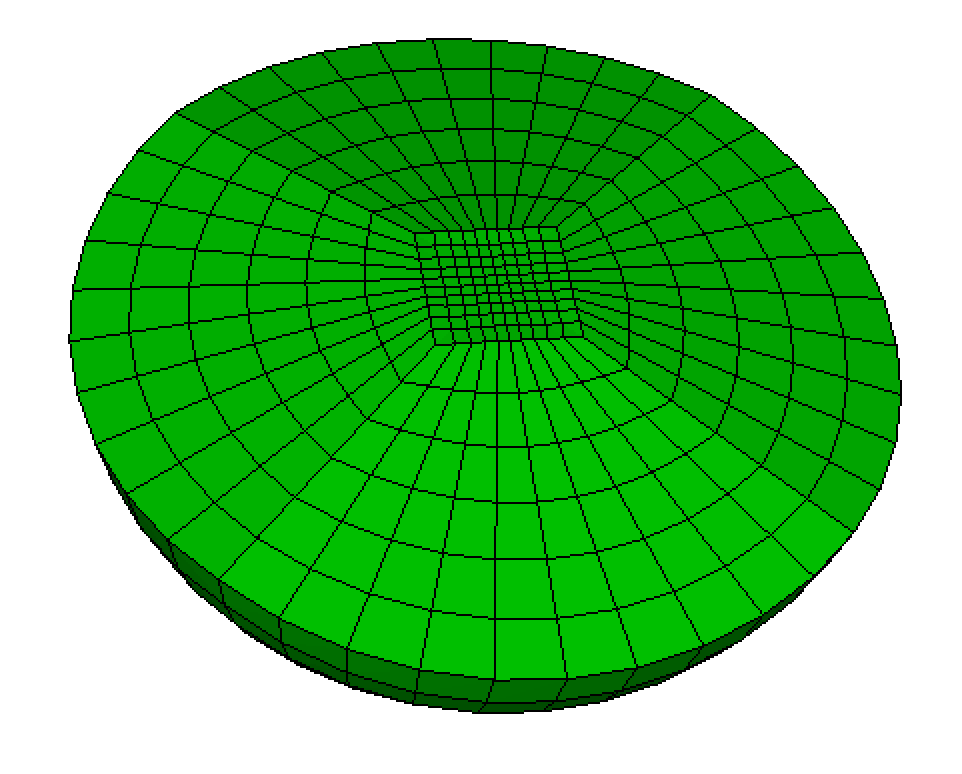
Figure 327:
FRACTION: fraction 0.7 graded_interval 6 az_interval 40 bias 1.0 max_smooth_iterations 0
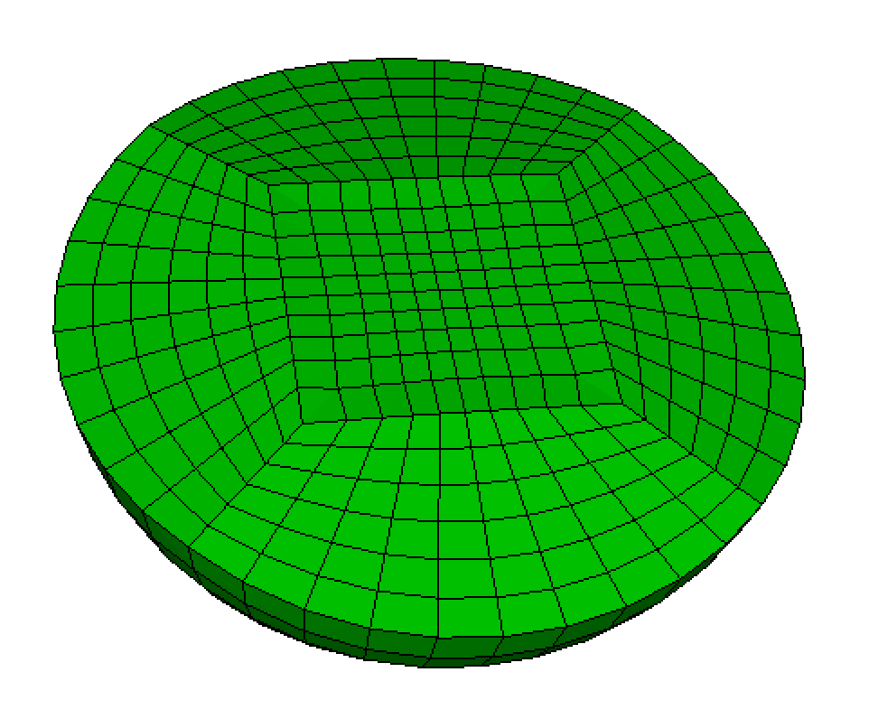
Figure 328:
INTERVAL: fraction 0.7 graded_interval 9 az_interval 40 bias 1.0 max_smooth_iterations 0
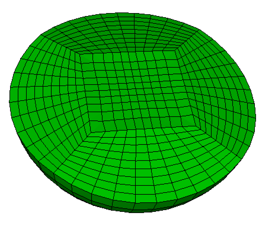
Figure 329:
SMOOTHING: fraction 0.7 graded_interval 9 az_interval 40 bias 1.0 max_smooth_iterations 2
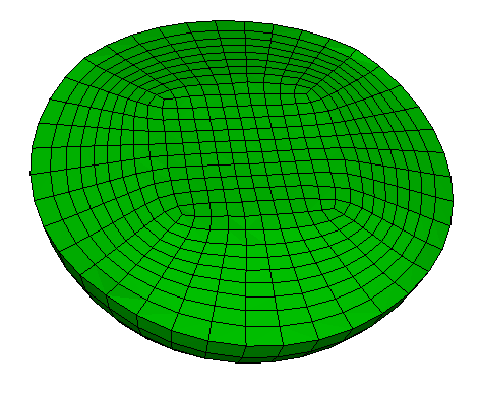
Figure 330:
AZIMUTHAL (mesh coarseness): fraction 0.7 graded_interval 5 az_interval 32 bias 1.0 max_smooth_iterations 2
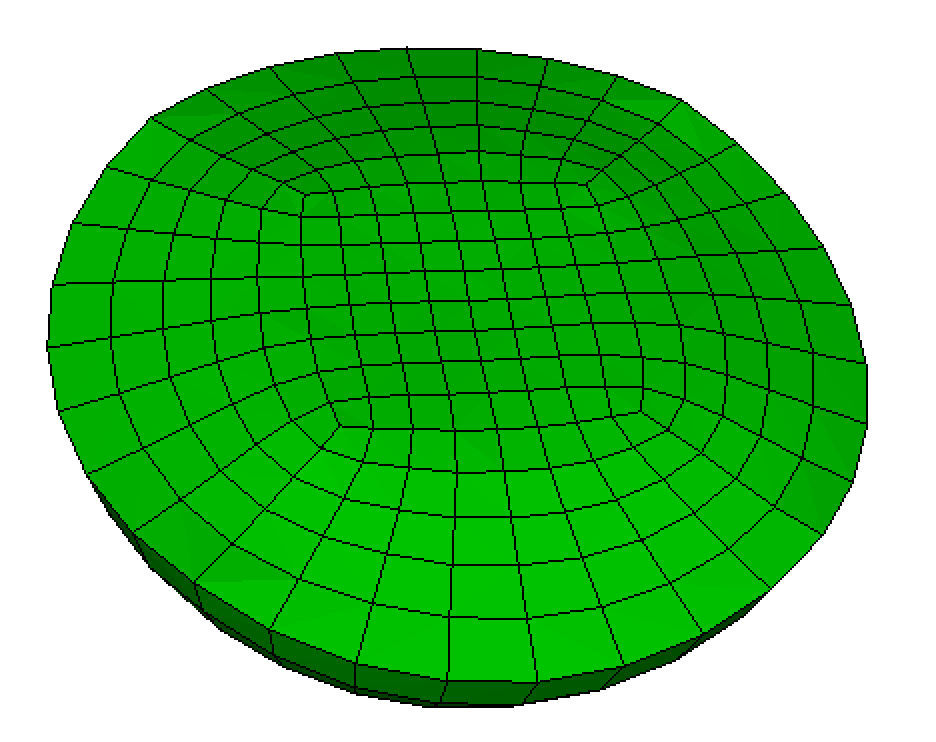
Figure 331:
BIAS (graded): fraction 0.9 graded_interval 9 az_interval 32 bias 1.5 max_smooth_iterations 0
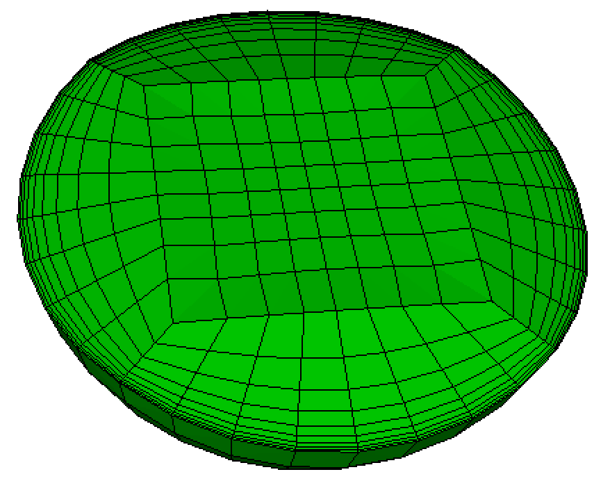
5.4.12.13 STransition
Applies to: Surfaces
Summary:
Produces a simple transitional mapped mesh.
Surface <surface_id_range> Scheme STransition [Triangle] [Coarse]
Discussion: The STransition scheme transitions a mesh from one element density to another across a surface. This scheme is particularly helpful when the Paving scheme produces a poor mesh. The following two figures show a specific case where the STransition scheme may offer an improvement.
| ||
|
The coarse option forces the mesh to transition to a coarser mesh in the first layer.
|
For triangular surfaces, the STransition scheme with the triangle option will produce similar results when compared to the Triprimitive scheme. However, STransition is capable of handling more varied interval settings. The following triangle fails when using the Triprimitive scheme but succeeds with the STransition scheme.
|
The figures below show the STransition meshing scheme response to different shapes and interval settings.
| |
|
The user also has the option of specifying END or SIDE surface vertex types.
|
Note, that the Centroid Area Pull smoothing algorithm sometimes gives better results than the default Winslow smoothing algorithm for STransition meshes.
5.4.12.14 Stretch
Applies to: Curves
Summary: Permits user to specify the exact size of the first and/or last edges on a curve.
To stretch a curve
On the Command Panel, click on Mesh and then Curve.
Click on the Mesh action button.
Enter the values for Select Curves. This can also be done using the Pick Widget function.
Select Stretch from the drop-down menu.
Select Size or Stretch Factor from the Size/Stretch menu.
Enter in the appropriate settings.
Click on Apply Size and then Mesh.
Curve <range> Scheme Stretch [First_size <double>] [Last_size <double>] [Start Vertex <id>]
Curve <range> Scheme Stretch [Stretch_factor <double>] [Start Vertex <id>]
Related Commands: Scheme Bias and Dualbias.
Discussion: This scheme allows the user to specify the exact length of the first and/or last edge on a curve mesh. Intermediate edge lengths will vary smoothly between these input values. Reasonable values for these parameters should be used (for example, the sizes must be less than the total length of the curve). If last_size is input, first_size must be input also. If stretch_factor is input, neither first_size nor last_size can be input. This scheme does not currently work on periodic curves.
5.4.12.15 Stride
Applies to: Curves
Summary: Mesh a curve with node spacing based on a general field function.
Curve <range> Scheme Stride
Discussion: The ability to specify the number and location of nodes based on a general field function is also available in Cubit. With this capability the node locations along a curve can be determined by some field variable (e.g. an error measure). This provides a means of using Cubit in adaptive analyses. To use this capability, a sizing function must have been read in and associated to the geometry (See Exodus II -based field function for more information on this process). After a sizing function is made available, the stride scheme can be used to mesh the curves.
5.4.12.16 Submap
Applies to: Surfaces, Volumes
Summary: Produces a structured mesh for surfaces/volumes with more than 4/6 logical sides
To submap on a surface
On the Command Panel, click on Mesh and then Surface.
Click on the Mesh action button.
Enter the values for Select Surface. This can also be done using the Pick Widget function.
Select SubMap from the drop-down menu.
Optionally, click on Advanced to further specify the settings.
Click on Apply Scheme and then Mesh.
To submap on a volume
On the Command Panel, click on Mesh and then Volume.
Click on the Mesh action button.
Enter the values for Select Volumes. This can also be done using the Pick Widget function.
Select SubMap from the drop-down menu.
Click on Apply Scheme and then Mesh.
{Surface|Volume} <range> Scheme Submap
Related Commands:
{Surface|Volume} <range> Submap Smooth <on|off>
Discussion: Submapping (Whiteley, 96) is a meshing tool based on the surface mapping capability discussed previously, and is suited for mesh generation on surfaces which can be decomposed into mappable subsurfaces. This algorithm uses a decomposition method to break the surface into simple mappable regions. Submapping is not limited by the number of logical sides in the geometry or by the number of edges. The submap tool, however is best suited for surfaces and volumes that are fairly blocky or that contain interior angles that are close to multiples of 90 degrees.
An example of a volume and its surfaces meshed with submapping is shown in Figure 332.

Volume submapping uses the logical sides for the bounding surfaces and the vertex types to construct a logical "i-j-k" coordinate system, which is used to construct the logical sides of the volume. For surface and volume submapping, the sides are used to formulate the interval constraints for the surface or volume.
Figure 333 shows an example of this logical classification technique, where the edges on the front surface have been classified in the i-j coordinate system; the figure also shows the submapped mesh for that volume.

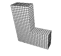
Set Submap CornerPicking {ON|off}
{Surface|Volume} <range> Submap Smooth <on|off>
Surface submapping also has the ability to mesh periodic surfaces such as cylinders. An example of a periodic surface meshed with submapping is shown in Figure 334. The requirement for meshing these surfaces is that the top and bottom of the cylinder must have matching intervals.

5.4.12.17 Surface Vertex Types
Several meshing algorithms in CUBIT "classify" the vertices of a surface or volume to produce a high quality mesh. This classification is based on the angle between the edges meeting at the vertex, and helps determine where to place the corners of the map, submap or trimesh, or the triangles in the trimap or tripave schemes. For example, a surface mapping algorithm must identify the four vertices of the surface that best represent the surface as a rectangle. Figure 335 illustrates the vertex angle types for mapped and submapped surfaces, and the correspondence between vertex types and the placement of corners in a mapped or submapped mesh.
Figure 335: Angle Types for Mapped and Submapped Surfaces: An End vertex is contained in one element, a Side vertex two, a Corner three, and a Reversal four.

The surface vertex type is computed automatically during meshing, but can also be specified manually. In some cases, choosing vertex types manually results in a better quality mesh or a mesh that is preferable to the user. Vertex types have a firmness, just as meshing schemes do. Automatically selected vertex types are soft, while user-set vertex types are hard. Instead of a type, an angle in degrees can be specified instead.
5.4.12.17.1 Surface Vertex Commands
Surface <surface_id> [Vertex <vertex_id_range> [Loop_index <int>]] Type {End|Side|Corner|Reversal}
Surface <surface_id> [Vertex [<vertex_id_range> [Loop_index <int>]] Angle <value>
Surface <surface_id> [Vertex <vertex_id_range> [Loop_index <int>]] Type {Default|Soft|Hard}
If no vertices are specified, the command is applied to all vertices of each surface. The loop_index is used only for vertices that are on the boundary of a single surface more than once.
Note that a vertex may be connected to several surfaces and its classification can be different for each of those surfaces.
The influence of vertex types when mapping or submapping a surface is illustrated in Figure 336. There, the same surface is submapped in two different ways by adjusting the vertex types of ten vertices.


Figure 336: Influence of vertex types on submap meshes; vertices whose types are changed are indicated above, along with the mesh produced; logical submap shape shown below.

5.4.12.17.2 Listing and Drawing Vertex Types
Draw Surface <surface_id_range> {Vertex Angle|Vertex Type}
5.4.12.17.3 Triangle Vertex Types
Surface <surface_id_range> Angle <angle>
Surface <surface_id> Set [Vertex <vertex_id_range> [Loop_index <int>]] Type {Triangle|Nontriangle}
5.4.12.17.4 Adjusting the Automatic Vertex Type Selection Algorithm
Set {Corner|End} Angle <degrees>
Set Corner Weight <value>
Set Turn Weight <value>
Set Interval Weight <value>
Set Large Angle Weight <value>
An illustration of a mesh produced by the submapping algorithm is shown in Figure 2. The meshes produced by submapping on the left and right result from adjusting the vertex types of the eight vertices shown.
5.4.12.17.5 Volume Curve Types
Draw Volume <surface_id_range> {Curve Angle|Curve Type}
List Volume <volume_id> Curve Type
Volume <volume_id> [Curve <curve_id_range>] Type {End|Side|Corner|Reversal}
Volume <volume_id> [Curve <curve_id_range>] Type {Default|Soft|Hard}
5.4.12.18 Sweep
Applies to: Volumes
Summary: Produces an extruded hexahedral mesh for 2.5D volumes.
Volume <range> Scheme Sweep [Source [Surface] <range>] [Target [Surface] <range>] [Propagate_bias] [Sweep_smooth {auto | smart_affine | linear | residual | winslow}] [Sweep_transform {LEAST_SQUARES | Translate}] [Autosmooth_target {ON|off}]
Volume <range> Scheme Sweep Vector <xval yval zval>
Volume <range> autosmooth_target [off|ON]
fixed_imprints [on|OFF]
smart smooth [ON|off] tolerance <val 0.0 to 1.0=0.2>
nlayers <val >=0=5>
Set Multisweep [On|Off]
Multisweep Smoothing {ON|Off}
Multisweep Volume <range> Remove
[Set] Legacy Sweeper {On|Off}
Discussion: The sweep algorithm can sweep general 2.5D geometries and can also do pure translation or rotations. A 2.5D geometry is characterized by source and target surfaces which are topologically similar. The hexahedral mesh is swept (extruded) between source and target along a single logical axis. Bounding the swept hexahedra between source and target surfaces, are the linking surfaces. Figures 1 and 2 show examples of source, target and linking surfaces.
Command Options: The user can specify the source and target surfaces. The user can also specify a geometric vector approximating the sweep direction, and let CUBIT determine the source and target surfaces. The user can specify just the source surfaces, and let cubit guess the target, or "scheme auto" can also be used.
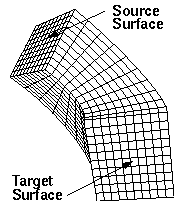
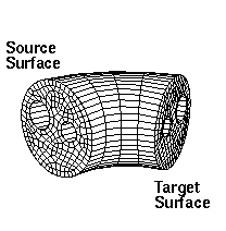
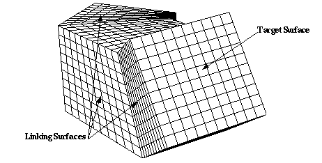
In many cases auto-scheme selection can simplify this process by recognizing sweepable geometries and automatically select source and target surfaces. If the source and target surfaces are not specified, CUBIT attempts to automatically select them. CUBIT also automatically sets curve and vertex types in an attempt to make the mesh of the linking surfaces lead from a source surface to a target surface. These automatic selections may occasionally fail, in which case the user must manually select the source/target surfaces, or some of the curve and vertex types. After making some of these changes, the user should again set the volume scheme to sweep and attempt to mesh.
Occasionally the user must also adjust intervals along curves, in addition to the usual surface interval matching requirements. For a given pair of source/target surfaces, there must be the same number of hexahedral layers between them regardless of the path taken. This constrains the number of edges along curves of linking surfaces. For example, in Figure 340 right, the number of intervals through the holes must be the same as along the outer shell.
Propagate_bias Option: The propagate_bias option attempts to preserve the source bias by propagating bias mesh schemes from the curves of the source surface to the curves of the target surface.
Sweep_transform Option: Swept meshes are created by projecting points between the source and target surfaces using affine transformations and then connecting them to form hexahedra. The method used to calculate the affine transformations is set using the sweep_transform option.
Least_squares: If the least_squares option is selected then affine transformations between the source and target are calculated using a least squares method.
translate: If the translate option is selected then a simple translate affine transformation is calculated based upon the centroid of the source and target.
Sweep_smooth Option: This option is available only in Legacy mode. The command set legacy sweeper on|off controls the mode. Legacy mode is OFF by default.
To ensure adequate mesh quality, optional smoothing schemes are available to reposition the interior nodes. The sweep tool permits five types of smoothing that are set with the following command prior to meshing a volume whose mesh scheme is sweep:
Linear: If this option is selected, no layer smoothing is performed. The node positions are determined strictly by the affine transformation from the previous layer. Good quality swept meshes can be constructed using "linear" provided the volume geometry and meshed linking surfaces permit the volume mesh to be created by a translation, scaling, and/or rotation of the source mesh. Volumes for which this is nearly true may also produce acceptable quality with "linear". As one would expect, this option generates swept meshes more quickly than the other sweep smooth options. This option is rarely needed since the next option produces better results with little time penalty.
Smart_affine: The "smart_affine" option does minimal smoothing of the interior nodes. Affine transformations are used to project the source and target surfaces to the middle surface of the volume. The position of the middle surface nodes is the average of the projected nodes from the source and target surfaces. The error in projecting from source and target is computed, and this error is linearly distributed back to the source and target.
Residual: The "residual" method is often used for meshing volumes that cannot be swept with the "smart linear" method. It tends to produce better quality meshes than the "smart linear" method while running faster than the Winslow-based smoother. The sweeping algorithm uses an affine transformation to calculate the interior nodes’ positions, but the mesh on the linking surface determines the positions of the nodes on the boundary of the layer. For the "residual" method, CUBIT calculates corrective adjustments for interior nodes using the "residuals" from boundary nodes. The "residual" is defined as the distance between the boundary node’s position (as determined by the surface mesh) and the boundary node’s ideal position (as determined by the affine transformation of the previous layer). Cubit computes the residual forward from the source and backward from the target to get best the possible node position.
Winslow: Smooth scheme "winslow" smooths each layer using a weighted, elliptic smoother. The weights are computed from the source mesh; they help maintain any biased spacing that occurs on the source mesh. For example, one might want to use the "winslow" option if the source was a biased mesh that was created using scheme circle. The biasing of the outer elements of the source mesh may be destroyed if one of the other smooth options is used. The interior nodes are initially place using the residual method.
AUTO: This is the default for the sweep_smooth option. "auto" causes the Sweeper to automatically choose between "smart_affine" and "residual." Auto will choose "off" if the layer needs little or no smoothing or "residual" if it needs smoothing. Scheme "auto" does not guarantee that no negative Jacobians are produced. This option produces acceptable results in most cases. If it fails to produce a quality mesh, then choose one of the other sweep smooth options.
If none of these smooth schemes result in adequate mesh quality, one can consider trying one of the volume smoothing schemes such as condition number or mean ratio.
Autosmooth_target Option and Command
Volume <range> autosmooth_target [off|ON]
fixed_imprints [on|OFF]
smart smooth [ON|off] tolerance <val 0.0 to 1.0=0.2>
nlayers <val >=0=5>
Issuing the command "Volume <id> autosmooth_target off", or using these options in the sweep command, will project the source nodes onto the target without any subsequent smoothing to improve quality. The result is that the relative placement of the nodes on the target will be as close to identical as possible to the relative placement of the node on the sources. This should be used when sweeping models that are very thin, and smoothing of the target could result in significant skew introduced in the thin layers in the sweep. Axisymmetric models might also want to turn OFF the autosmooth_target so that the nodes are identically placed on the symmetry plane surfaces.
Issuing the command "Volume <id> autosmooth_target on", or using it as an option in the sweep command, will call a surface smoother after the initial projection of the nodes onto the target in order to improve surface element quality. This smoothing does not consider hex element quality, only quality of the target surface mesh. This command will smooth all nodes on the target surface. Adding the "fixed_imprint on" keyword onto the command will cause the target nodes which are projections of source nodes on source curves and vertices to remain fixed during smoothing. Only target nodes, which are projections of source surface nodes will be smoothed. The "smart smooth on" option provides further control to the user. If "smart smooth" is turned on, target surface smoothing will only move nodes which are within "nlayers" of a target surface quad element that has a scaled Jacobian quality measure less than the specified "tolerance" value.
5.4.12.18.1 Multisweep
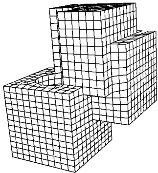
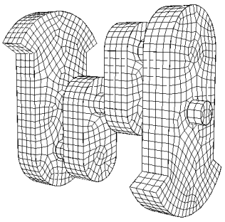
Linear: If this option is active and/or target surfaces are omitted from the scheme setting command, CUBIT will determine source and target surfaces (See Automatic Scheme Selection). Sweeping can be further automated using the "sweep groups" command.
Limitations: Not all geometries are sweepable. Even some that appear sweepable may not be, depending on the linking surface meshes. Highly curved source and target surfaces may not be meshable with the current sweep algorithm.
5.4.12.18.2 Grouping Sweepable Volumes
Swept meshing relies on the constraint that the source and target meshes are topologically identical or the target surface is unmeshed. This results in there being dependencies between swept volumes connected through non-manifold surfaces; these dependencies must be satisfied before the group of volumes can be meshed successfully. For example, if the model was a series of connected cylinders, the proper way to mesh the model would be to sweep each volume starting at the top (or bottom) and continuing through each successive connected volume.
With larger models and with models that contain volumes that require many source surfaces, the process of determining the correct sweeping ordering becomes tedious. The sweep grouping capability computes these dependencies and puts the volumes into groups, in an order which represents those dependencies. The volumes are meshed in the correct order when the resulting group is meshed.
Group Sweep Volumes
Mesh sweep_groups
Set {Source|Target} Surface Pattern ’<pattern>’ [Include Volume Name]
br x 10
surface 1 name ’brick.top’
surface 2 name ’brick.bottom’
set source surface pattern ’top’
set target surface pattern ’bottom’
volume 1 scheme sweep
list volume 1 brief
5.4.12.18.3 Node Redistribution
Volume <range> redistribute nodes {ON|off}
With redistribute set to ON, the boundary nodes of a mappable surface are moved until the spacing between the nodes are equivalent on the two opposing curves. In other words, the parametric values of the nodes lying on the two opposite curves are matched.
Redistribute option ON will assist in avoiding the skewness of the mapped mesh. In the below examples, the linking surfaces are meshed using mapped scheme, and with redistribute option ON, the skewness is significantly avoided (see figures (4) and (5)).
Note: 1. Redistribute option ON will affect all mapped surfaces, not just the linking surfaces of a swept volume. Even though the example below shows a swept volume, the command can be used independent of the sweeping command. That is, it can be used while meshing surface models that contain mappable surfaces.
2. If the linking surfaces of a swept mesh contain submappable surfaces, then the affect of redistribute option ON is generally not seen. The current implementation is restricted to mappable surfaces only and doesn’t handle submappable surfaces. In the future, we should be able to easily extend the redistribute option to submappable surfaces.
Figure 340: Linking surfaces of a many-to-one sweepable solid (shown in green) is mappable
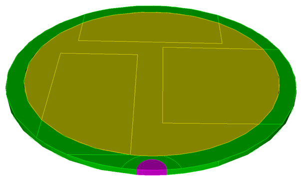
Figure 341: Highly skewed elements on the linking mapped surface with 'redistribute nodes OFF'
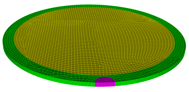
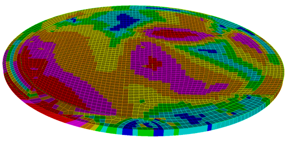
Figure 343: High skew on the linking mapped surface can be avoided with 'Redistribute Nodes ON'
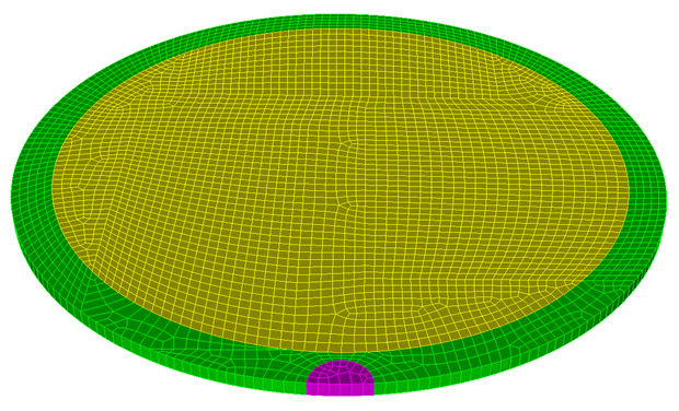
5.4.12.19 TetMesh
}
Applies to: Volumes
Summary: Automatically meshes a volume with an unstructured tetrahedral mesh.
Volume <range> Scheme TetMesh [Proximity Layers {on[<num_layers>]|OFF}] [Geometry Approximation Angle <angle>]
[Set] Tetmesher Add mid_edge_nodes {on|OFF}
[Set] Tetmesher Optimize Surface mid_edge_nodes {on|OFF}
[Set] Tetmesher Anisotropic layers {on|OFF [<layers=2>]}
[Set] Tetmesher Boundary Recovery {on|OFF}
[Set] Tetmesher HPC {on|OFF} [Threads <value=4>]
[Set] Tetmesher Interior Points {ON|off}
[Set] Tetmesher Optimize { { [Level} <level> [Overconstrained Edges {on|OFF}] [Overconstrained Tetrahedra {on|OFF}] [Sliver {on|OFF}] } | Default
[Set] Trimesher Surface Gradation <value>
[Set] Trimesher Volume Gradation <value>
[Set] Trimesher Geometry Sizing {ON|off}
[Set] Trimesher Split Overconstrained Edges {on|OFF}
THex Volume All
Volume <volume_id> Tetmesh Respect {Face|Tri|Edge|Node} <range>
Volume <volume_id> Tetmesh Respect Clear
Volume <volume_id> Tetmesh Respect File ’<filename>’
Volume <volume_id> Tetmesh Respect Location (options)
5.4.12.19.1 Discussion
The TetMesh scheme fills an arbitrary three-dimensional volume with tetrahedral elements. The surfaces are first triangulated with one of the triangle schemes (TriMesh, TriAdvance or TriDelaunay) or a quadrilateral scheme with the quadrilaterals being split into two triangles (QTri). If a meshing scheme has not been applied to the surfaces, the TriMesh scheme will be used.
Included in Cubit is a third party software library for generating tetrahedral meshes called MeshGems. This is a robust and fast tetrahedral mesher developed by the French laboratory INRIA and distributed by Distene. It utilizes an algorithm for automatic mesh generation based upon the Voronoi-Delaunay method. Figure 345 shows a CAD model meshed with the TetMesh scheme, with the TriMesh scheme used to mesh the surfaces.
(a)
(b)
(c)
(d)
Figure 345: Tetrahedral mesh generated with the TetMesh scheme using default settings. (a) Initial CAD geometry (b) CAD model with surface mesh generated with TriMesh scheme. (c) and (d) Cut-away views of the interior tetrahedral mesh
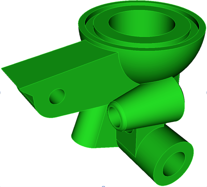
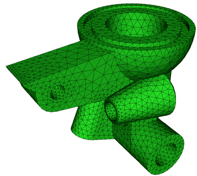
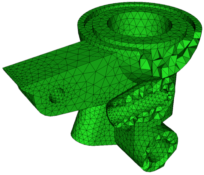
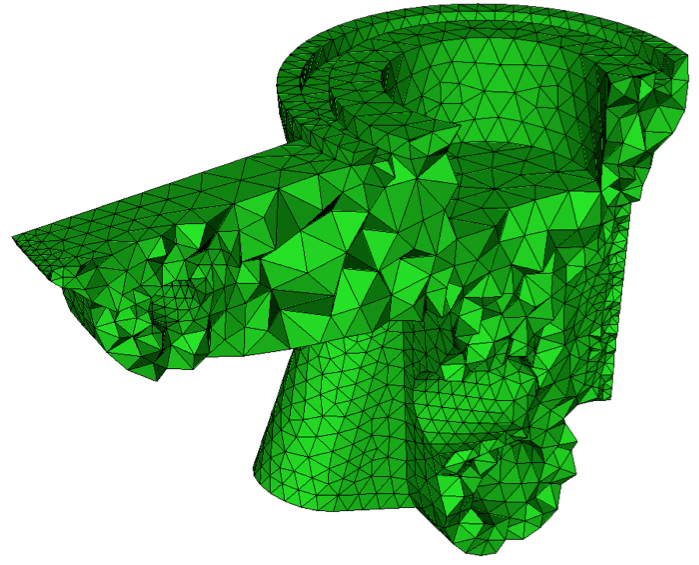
The TetMesh scheme is usually very good at generating a mesh with its default settings. In most cases no adjustments to default settings are necessary. Using the size assigned to the volume, either assigned explicitly or defined with an auto size, the TetMesh scheme will attempt to maintain the assigned size, except where features smaller than the specified size exist. In this case, smaller tets will automatically be generated to match the feature size. The tet mesher will then generate a smooth gradation from the small tets used to capture features, to the size specified on the volume. This effect is shown in figure 1 where internal transitions in tetrahedra size can be seen. User defined sizes and intervals can also be assigned to individual surfaces and curves for more specific control of element sizes.
A sizing function can also be used with the TetMesh scheme to control element sizes, however the algorithm used for meshing surfaces will automatically revert to the TriAdvance scheme. This is because the TetMesh scheme provides built-in capabilities for adaptively controlling the element sizes based on geometry. More details can be found in Geometry Adaptive Sizing for TriMesh and TetMesh Schemes
When using the TetMesh and TriMesh schemes, recommended practice is to mesh all surfaces and volumes simultaneously. This provides the greatest flexibility to the algorithms to determine feature sizes and their effect on neighboring surfaces and volumes.
5.4.12.19.2 TetMesh Scheme Options
Proximity Layers {on[<num_layers>]|OFF}
In some thin regions of the model, it may be necessary to ensure a minimum number of element layers through the thickness to better capture physical properties. Using the proximity layers setting, the specified minimum num_layers of tetrahedra will be placed in thin regions, even if the tetrahedra sizes drop below the size assigned to the volume. The default setting for proximity layers is OFF where element sizes will not be affected in thin regions.
Figure 346: Demonstrates the effect of using proximity layers on a cut-away section of a volume. Note the layers of smaller tets placed in the thin region.
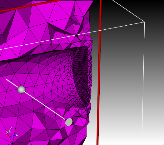
Geometry Approximation Angle <angle>
For non-planar CAD surfaces, an approximation must always be made to capture the curved features using the linear faces of the tetrahedra. When a geometry approximation angle is specified, the tet mesher will adjust element sizes on curved surfaces so that the linear edges of the tetrahedra will deviate no greater than the specified angle from the geometry. Figure 347 illustrates how the geometry approximation angle is determined. If the red curve represents the geometry and the black segments represent the mesh, the angle θ is the angle between the tangent plane at point A and the plane of a triangle at A. θ represents the maximum deviation from the geometry that the mesh will attempt to capture. As shown in figure 2(b), a smaller geometry approximation angle will normally result in more elements, but it will more closely approximate the actual geometry. The default approximation angle is 15 degrees.
(a)
(b)
Figure 347: The geometry approximation angle θ is shown as the maximum deviation between the tangent plane at A and the plane of a triangle at A.
Figure 348: Demonstrates the effect of the geometry approximation angle set on the volume. Triangle sizes on the interior of surfaces will be adjusted to better capture curvature.
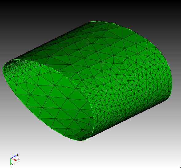
5.4.12.19.3 Global Tetmesher Options
[Set] Tetmesher Add mid_edge_nodes {on|OFF}
[Set] Tetmesher Optimize Surface mid_edge_nodes {on|OFF}
[Set] Tetmesher Anisotropic Layers {on|OFF [<layers=2>]}
The anisotropic layers setting attempts to place the specified number of layers of tetrahedra through thin regions of the volume while respecting the volume mesh size in the thick direction. The default number of layers is two. This option is currently under development and can sometimes generate high aspect ratio tetrahedra. The number of layers generated can sometimes exceed the number of layers specified..
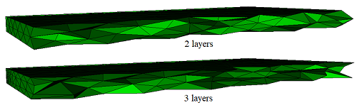
[Set] Tetmesher Boundary Recovery {on|OFF}
[Set] Tetmesher HPC {on|OFF} [Threads <value=4>]
[Set] Tetmesher Interior Points {ON|off}
[Set] Tetmesher Optimize Level <level>
[Set] Tetmesher Optimize Overconstrained Edges {on|OFF}
[Set] Tetmesher Optimize Overconstrained Tetrahedra {on|OFF}
[Set] Tetmesher Optimize Sliver {on|OFF}
[Set] Tetmesher Optimize Default
The tetmesher optimize default command restores the default optimization values: level = 3 (standard), overconstrained edges = off, overconstrained tetrahedra = off, and sliver = off.
5.4.12.19.4 Using tets as the basis of an unstructured hexahedral mesh
Tet meshing can be used to generate hexahedral meshes using the Thex command. Each of the tetrahedron can be converted into 4 hexes, producing a fully conformal hexahedral mesh, albeit of poorer quality. These meshes can often be used in codes that are less sensitive to mesh quality and mesh directionality. The Thex command requires that all tets in the model be converted to hexahedra with the same command.
5.4.12.19.5 Conforming the tetmesh to internal features
Volume <volume_id> Tetmesh Respect {Face|Tri|Edge|Node} <range>
The tetmesh respect command allows the user to specify mesh entities that will be part of a tetrahedral mesh. These faces, triangles, edges, or nodes are inside the volume since all surface mesh features will appear in the final tetrahedral mesh by default. These mesh entities specified to be respected can be generated from other meshing commands on free vertices, curves, or surfaces.
Figure 350: Example of using tetmesh respect to ensure node 9 is captured in the tetmesh.
volume 1 scheme tetmesh
tetmesh respect node 9
mesh volume 1
volume 3 scheme tetmesh
volume 3 tetmesh respect node 12
volume 3 tetmesh respect tri 2
mesh volume 1
Volume <volume_id> Tetmesh Respect File ’<filename>’
Volume <volume_id> Tetmesh Respect Location (options)
volume 1 tetmesh respect location 1 0 -1
This is much simpler than creating the vertex, meshing it, and then respecting it.
volume 2 tetmesh respect file ’my_points.facet’
Volume <volume_id> Tetmesh Respect Clear
The tetmesh respect clear command is the only way to remove respected data from a volume without deleting the volume. Unfortunately, it removes all respected data from the volume. Therefore, if the model has a lot of data to be respected, it is best to put it in a file or keep a journal file that can be edited.
5.4.12.19.6 Controlling the gradation of the mesh size inside the volume
Volume <id_range> Tetmesh growth_factor <value 1.0 to 10.0 = 1.05>
The growth_factor option controls how fast the tetrahedra sizes can change when transitioning from small to larger sizes within the volume. For example a value of 1.5 will attempt to limit the ratio between 2 adjacent tetrahedral edges. Valid values for gradation should be greater than or equal to 1.0 and usually less than 2 or 3. The larger the value, the faster the transition is. Likewise, values closer to 1.0 will result in a more uniform mesh. The default setting for growth_factor is 1.05, allowing for a somewhat slow transition between sizes within a volume. The size at the interior of a volume can be controlled using the volume <range> [interval] size <interval_size> command.
Gradation of the triangles on the surfaces can also be controlled independently using the global settings [set] trimesher surface gradation and [set] trimesher volume gradation.
5.4.12.19.7 Generating a Tetmesh from a Skin of Triangles
Tetmesh Tri <ids> [growth_factor <value>] [Make {Block|Group} [<id>]]
Tetmesh Tri <ids> [growth_factor <value>] {Add|Replace} {Block <id>|Group <id>}
The tetmesh tri command generates a tetrahedral mesh from the list of triangles entered. The triangles must form a closed surface. The command fails if they do not. The list of triangles may be a skin, and thus a command such as tetmesh tri in block 1 would be acceptable, should block 1 be a previously defined skin.
The first command form has optional arguments. If the make option and its arguments are present, then the specified block or group will contain the generated tet elements. The command fails with the make option if the specified block or group already exists. If the block or group id is omitted, the next available block or group id is used.
The second command form has two options, add and replace. Each option requires specifying an existing block or group. If the block or group does not exist, the command fails. The add option appends the tet elements to the block or group. The replace option removes any existing mesh from the block or group before adding the tet elements.
The growth_factor option helps control the transition from small to larger sizes within the mesh. The value specified will be the approximate ratio in the size of adjacent tets going from the boundary into the interior of the mesh. For example, a growth_factor of 1.0 will give near-constant sizing, while a growth_factor of 1.3 allows approximately 30% growth in each layer of adjacent tets.
5.4.12.20 Tetprimitive
Applies to: Volumes
Summary: Meshes a 4 "sided" object with hexahedral elements using the standard tetrahedron primitive.
To use a tetprimitive scheme
On the Command Panel, click on Mesh and then Volume.
Click on the Mesh action button.
Enter the appropriate value for Select Volumes. This can also be done using the Pick Widget function.
Select Tetprimitive from the drop-down menu.
Enter the appropriate settings.
Click Apply Scheme.
Click Mesh.
Volume <range> Scheme Tetprimitive [Combine Surface <range>] [Combine Surface <range>] [Combine Surface <range>] [Combine Surface <range>]
Discussion: The tetprimitive scheme is used to create a hexahedral mesh in a volume which fits the shape of a tetrahedral primitive. The Tetprimitive scheme assumes that each of the four surfaces have been meshed with the triprimitive, or similar, meshing scheme. If more than four surfaces form the tetrahedron geometry, the surfaces forming a logical side can be combined using the combine option.
Figure 351: Sphere octant hex meshed with scheme Tetprimitive, surfaces meshed using scheme Triprimitive
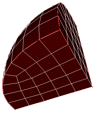
5.4.12.21 TriAdvance
Applies to: Surfaces
Summary: Automatically meshes surface geometry with triangle elements.
surface <range> scheme triadvance
Discussion: The triangle meshing scheme TriAdvance fills an arbitrary surface with triangle elements. It is an advancing front algorithm which allows holes in the surface and transitions between dissimilar element sizes. It can use a sizing function like the pave scheme if one is defined for the surface. Future development will add hard lines to this scheme’s capabilities. You specify this scheme for a surface by giving the command:
5.4.12.22 TriDelaunay
Applies to: Surfaces
Summary: Automatically meshes parametric surface geometry with triangle elements.
To use a tridelaunay scheme
On the Command Panel, click on Mesh and then Surface.
Click on the Mesh action button.
Enter the appropriate value for Select Surfaces. This can also be done using the Pick Widget function.
Select TriDelaunay from the drop-down menu.
Click Apply Scheme then click Mesh.
Surface <range> Scheme TriDelaunay
[Set] Tridelaunay point placement {gq | guaranteed quality | asp}
This algorithm is unstable for periodic surfaces which include a singularity point, E.G. spheres with poles, cone tips and some types of toruses.Use scheme TriMesh, TriAdvance or QTri to mesh non-parametric or periodic parametric surfaces.
5.4.12.23 TriMap
Applies to: Surfaces
Summary: Places triangle elements at some vertices, and map meshes the remaining surface.
Surface <range> Scheme Trimap
Surface <range> Vertex <range> Type {Triangle|Notriangle}
Discussion: Some surfaces contain bounding curves which meet at a very acute angle. Meshing these surfaces with an all-quadrilateral mesh will result in a very skewed quad to resolve that angle. In some cases, this is a worse result than simply placing a triangular element to resolve that angle. This scheme resolves this situation by placing a triangular element in these tight corners, and filling the remainder of the surface with a mapped mesh.
Surface <range> Vertex <range> Type {Triangle|Notriangle}
5.4.12.24 TriMesh
Applies to: Surfaces
Summary: Automatically meshes surface geometry with triangle elements using the third part meshgems tool.
Surface <range> Scheme TriMesh [Geometry Approximation Angle <angle>] [Meshgems] [Minimum Size <value>]
[Set] Trimesher Surface Gradation <value>
[Set] Trimesher Volume Gradation <value>
[Set] Trimesher Geometry Sizing {ON|off}
[Set] Trimesher Split Overconstrained Edges {on|OFF}
[set] trimesher ridge_angle {value=100}
Discussion: The TriMesh scheme fills a surface of arbitrary shape with triangle elements. The TriMesh scheme serves as the default method for meshing the surfaces of volumes for the TetMesh scheme.
Included in Cubit is a third party software library for generating triangle meshes called MeshGems. This is a robust and fast triangle mesher developed and distributed by Distene. Figure 352 shows a CAD model where surfaces have been meshed with the TriMesh scheme. The triangle mesh was then used as input to the TetMesh scheme.
Figure 352: Triangle meshes generated with the TriMesh scheme using default settings on the surfaces of a CAD model.
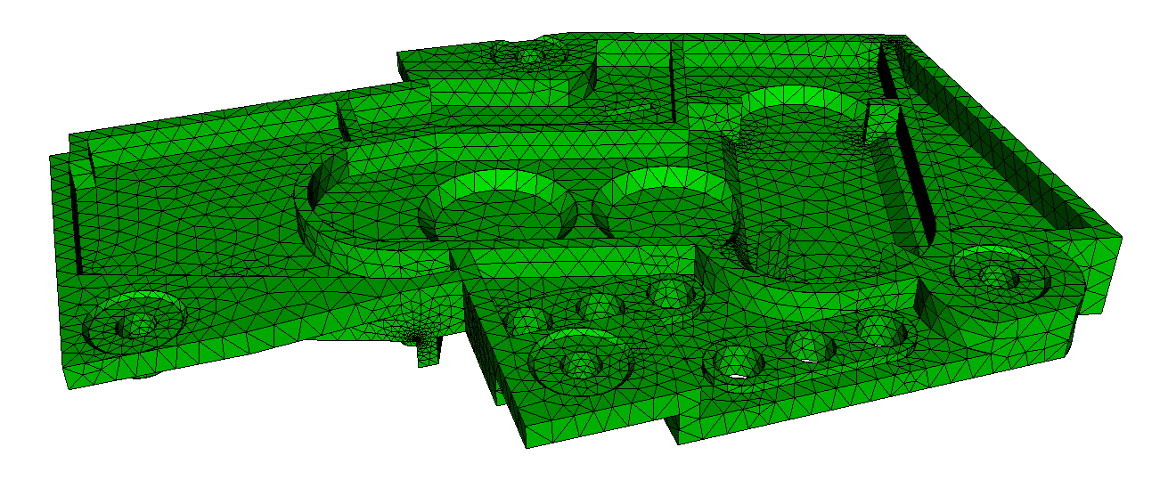
Although rare, if meshing fails when using the TriMesh scheme, Cubit will automatically attempt to mesh the surface with the TriDelaunay scheme. Subsequent mesh failures will also attempt meshing with the TriAdvance and QTri schemes.
A sizing function can also be used with the TriMesh scheme to control element sizes, however the algorithm used for meshing will automatically revert to the TriAdvance scheme. This is because the MeshGems algorithm provides built-in capabilities for adaptively controlling the element sizes based on geometry. More details can be found in Geometry Adaptive Sizing for TriMesh and TetMesh Schemes
When using the TriMesh and TetMesh schemes, recommended practice is to mesh all surfaces and volumes simultaneously. This provides the greatest flexibility to the algorithms to determine feature sizes and their effect on neighboring surfaces and volumes.
5.4.12.24.1 TriMesh Scheme Options
Geometry Approximation Angle <angle>
For non-planar CAD surfaces and non-linear curves, an approximation must always be made to capture the curved features using the linear edges of the triangle. When a geometry approximation angle is specified, the triangle mesher will adjust triangle sizes on curved boundaries so that the linear edges of the triangle will deviate from the geometry by no greater than the specified angle. Figure 353 illustrates how the geometry approximation angle is determined. If the red curve representes the geometry and the black segments represent the mesh, the angle θ is the angle between the tangent plane at point A and the plane of a triangle at A. θ represents the maximum deviation from the geometry that the mesh will attempt to capture. As shown in figure 2(b), a smaller geometry approximation angle will normally result in more elements, but it will more closely approximate the actual geometry. The default approximation angle is 15 degrees.
(a)
(b)
Figure 353: The geometry approximation angle θ is shown as the maximum deviation between the tangent plane at A and the plane of a triangle at A.
Note that the geometry approximation angle is also effective in controlling the element size on the interior of surfaces as illustrated in figure 3. This is most useful when used in conjunction with the TetMesh Scheme where smaller tets will be placed in regions of higher curvature.
Figure 354: Demonstrates the effect of the geometry approximation angle to better capture surface curvature on the interior of surfaces.
Minimum Size <value>
By specifying a minimum size, the tri mesher will attempt to prevent creating elements smaller than this specified size. It should be noted that there may still be a small number of elements with a size slightly less that this value; it is not an exact setting.
The meshgems option will use only the MeshGems triangle mesher on the specified surfaces. It will not revert upon failure to the TriDelaunay or TriAdvance schemes.
5.4.12.24.2 Global Trimesher Gradation Options
The user may set options that control the gradation of the tri-meshing algorithms. These trimesher options are global settings and apply to all trimeshes generated when the scheme is set to TriMesh until the option is changed by the user.
[Set] Trimesher Surface Gradation <value>
surface gradation will control the growth of triangles where element size has been determined by bounding curves. For example, Figure 355 shows a small feature where element sizes have been determined locally by the length of the small curves. A gradation is applied so that triangle sizes increase away from the small feature. A surface gradation of 1.3 is shown on the left, while a surface gradation of 1.1 is shown on the right.
(a)
(b)
Figure 355: Demonstrates the effect of changing the default gradation, where (a) is the default gradtion of 1.3, compared with (b) using a gradation of 1.1. Note that both images use the same interval size setting for the surface.
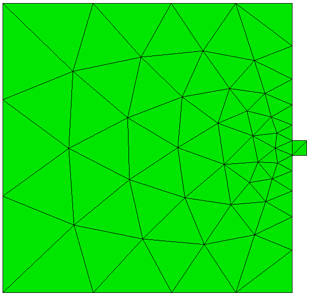
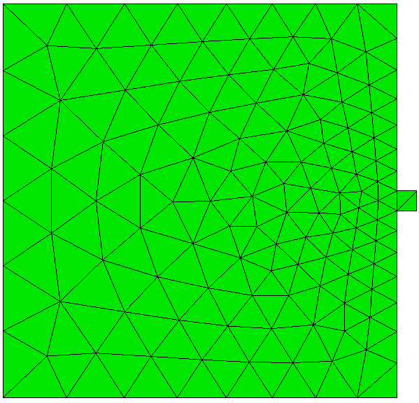
[Set] Trimesher Volume Gradation <value>
volume gradation will control the growth of triangles where element size has been determined by the proximity of other nearby surfaces. For example, Figure 357a and 5b shows a brick with a small void where the surface meshes are generated with the TriMesh scheme. The surface gradation has been adjusted to a large number so its effect is negligible. The small element size determined for the void is propagated to the exterior surfaces. The resulting gradation of the nearby triangles on the surface is determined by the trimesh volume gradation setting.
Note that the trimesh volume gradation command is different than the growth factor control setting. The trimesh volume gradation controls the gradation of triangles on the surface due to nearby features where small tets will exist, whereas the volume <range> tetmesh growth_factor command controls the gradation of the interior tet elements.
Figure 356: a. An example of a cut-away mesh with a volume gradation, where the small size on the interior void propagates to the exterior surfaces
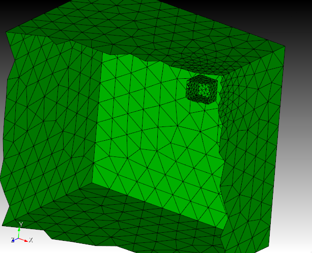
Figure 357: a. An example of a cut-away mesh with a volume gradation, where the small size on the interior void propagates to the exterior surfaces
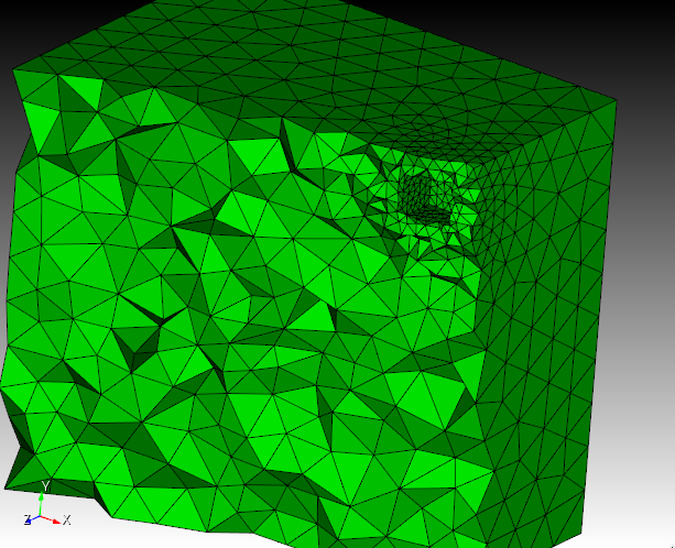
[Set] Trimesher Geometry Sizing {ON|off}
The global geometry sizing option can be toggled on or off. If set to on, the element size will be influenced by the geometry approximation angle. If set to off, geometry approximation angle will not be involved in the computation of element size. See geometry approximtion angle for more information.
[Set] Trimesher Split Overconstrained Edges {on|OFF}
The global split overconstrained edges, if set to on, splits edges owned by the surface, but with both nodes on curves. This feature can help when two elements through the thickness of the mesh is desired. Figure 358 shows the effect of this option.
[set] trimesher ridge_angle {value=100}

5.4.12.25 TriPave
Applies to: Surface
Summary: Places triangle elements at some vertices, and paves the remaining surface.
Surface <range> Scheme Tripave
Surface <range> Vertex <range> Type {triangle|notriangle}
Discussion: Similar to the trimap algorithm, but uses paving instead of mapping to fill the remainder of the surface with quadrilaterals.
Surface <range> Vertex <range> Type {triangle|notriangle}
5.4.12.26 TriPrimitive
Applies to: Surfaces
Summary: Produces a triangle-primitive mesh for a surface with three logical sides
To use a triprimitive scheme
On the Command Panel, click on Mesh and then Surface.
Click on the Mesh action button.
Enter the appropriate value for Select Surfaces. This can also be done using the Pick Widget function.
Select TriPrimitive from the drop-down menu.
Click Apply Scheme then click Mesh.
Surface <range> Scheme Triprimitive [SMOOTH | nosmoothing]
Discussion: The triprimitive scheme indicates that the region should be meshed as a triangle. A surface may use the triprimitive scheme if three "natural", or obvious, corners of the surface can be identified. For instance, the surface of a sphere octant (shown in the figure below) is handled nicely by the triprimitive scheme. The algorithm requires that there be at least 6 intervals (2 per side) specified on the curves representing the perimeter of the surface and that the sum of the intervals on any two of the triangle’s sides be at least two greater than the number of intervals on the remaining side. The following figure illustrates a triprimitive mesh on a 3D surface. By default, the triprimitive algorithm will smooth the mesh with an iterative smoothing scheme. This smoothing can be disabled by using the "nosmoothing" option with this command. The quality of the mesh will often be significantly degraded by disabling smoothing, but in certain cases the unsmoothed mesh may be preferred.